우리손 보조정리와 우리손 거리화 정리

09 Jul 2025

우리손 보조정리

우리손 보조정리_{Urysohn Lemma}. $X$가 정규_normal 공간이라고 하자. $A, B$가 서로소인 $X$의 닫힌집합일 때, 어떤 연속함수 $f: X \to [0, 1]$이 존재하여 $f[A] = \lbrace 0 \rbrace$, $f[B] = \lbrace 1 \rbrace$이다.

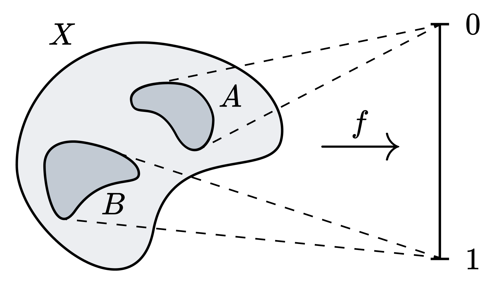
정규성을 비롯한 분리 공리는 해당 공간에서 점과 닫힌집합을 분리한다. 우리손 보조정리의 의의는, 정규성 분리 공리의 경우 두 닫힌집합은 좋은 공간에서도 분리 가능하다는 것이다. 구체적으로, 정규공간을 적절한 연속함수로 사상시켰을 때 두 닫힌집합은 $[0, 1]$에서 분리 가능하다. 그리고 $[0, 1]$의 여러 좋은 성질은 — 콤팩트 하우스도르프 거리 공간일 뿐 아니라 우리에게 굉장히 익숙한 공간이라 논증하기도 쉽다 — 우리손 보조정리의 굉장한 잠재력을 암시한다.

증명

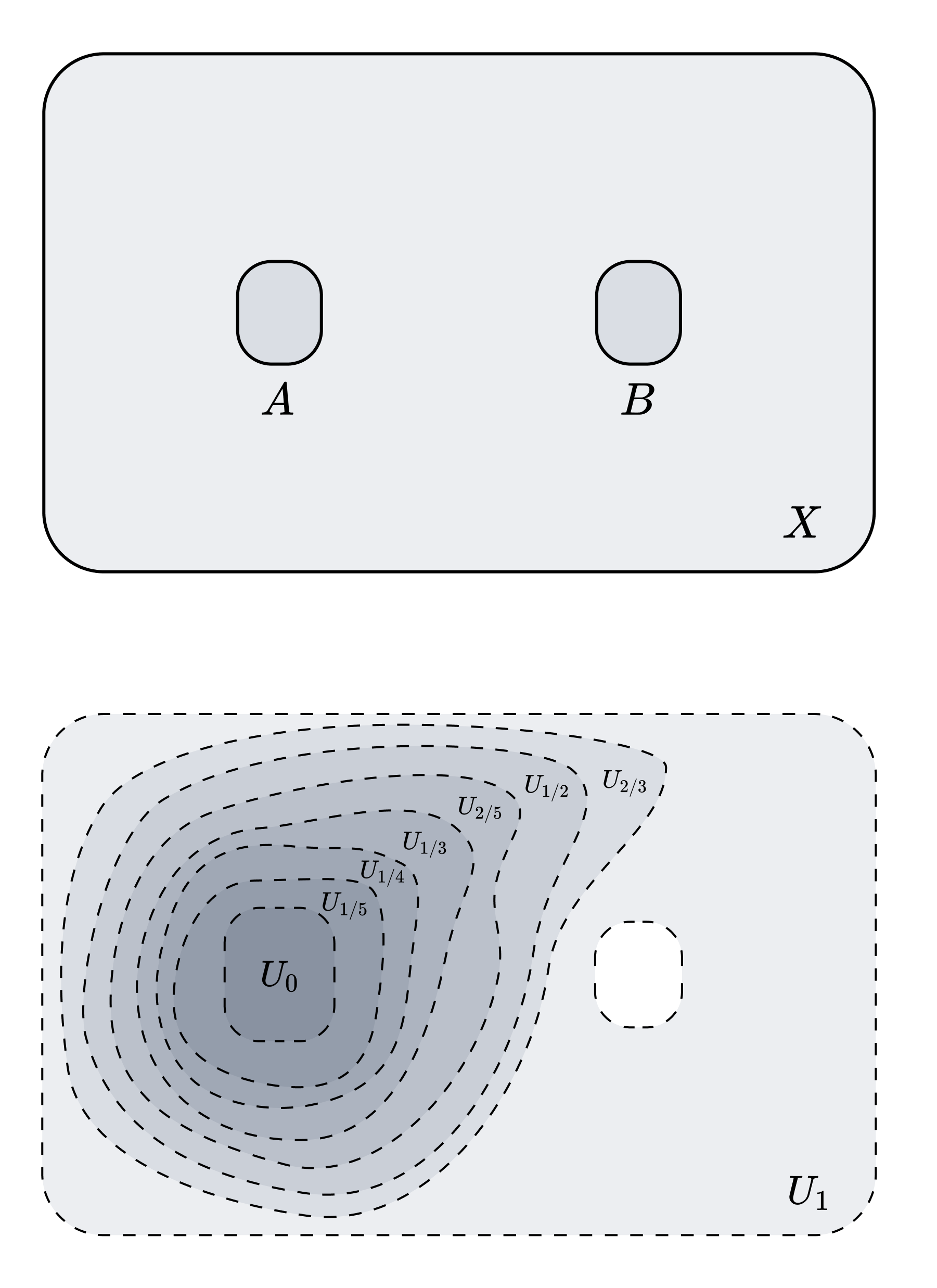
$Q = [0, 1] \cap \mathbb{Q}$라고 하자 (사실 $[0, 1]$의 가산 조밀 집합이기만 하면 된다). $Q$가 가산이므로 $Q$의 원소를 열거_enumerate하는 방법이 존재한다. 일례로 분모-분자의 사전식 열거 $\prec$를 고려하자.

\[0 \prec 1 \prec 1/2 \prec 1/3 \prec 2/3 \prec 1/4 \prec 1/5 \prec 2/5 \prec \cdots\]

이제 다음과 같이 $\lbrace U_q \rbrace _{q \in Q}$를 정의하자. 먼저 $U_1 = X \setminus B$이다 ($B$가 닫힌집합이므로 $U_1$은 열린집합이다). 정규성에 의해 $A \subset U_0$이면서 $\overline{U_0} \subset U_1$인 $U_0$가 존재한다. 나머지 $U_q$는 열거 순서에 따라 다음과 같이 정의한다. $p \prec q$인 임의의 $p$에 대해,

• $p < q \implies \overline{U_p} \subset U_q$
• $q < p \implies \overline{U_q} \subset U_p$

정규성에 의해 위 조건을 만족하며 $\lbrace U_q \rbrace _{q \in Q}$를 완전히 정의할 수 있다.

이제 다음과 같이 함수 $f: X \to [0, 1]$을 정의하자.

\[f(x) = \begin{cases} \sup_{<}\{q \in Q : x \notin U_q \} & x \notin U_0 \\ 0 & x \in U_0 \end{cases}\]

$\sup_<$라는 표기는 $\prec$가 아닌 $<$에 대해 상한을 취함을 의미한다. 정의로부터 $f[A] = 0, f[B] = 1$가 따라 나온다.

이제 $f$가 연속임을 보이면 정리가 증명된다. $\lbrace B_\epsilon(q) \cap [0, 1] : q \in Q, \epsilon \in \mathbb{Q}_{>0} \rbrace $가 $[0, 1]$의 위상 기저이므로, 임의의 $q \in Q$와 특정 상한보다 작은 양의 유리수 $\epsilon$에 대해 $S_{q, \epsilon} = f^{-1}(B_\epsilon(q) \cap [0, 1])$가 열린집합임을 보이면 충분하다.

• $0 < q < 1$인 경우, $S_{q, \epsilon} = (X \setminus \overline{U_{q-\epsilon}}) \cap U_{q + \epsilon}$이므로 열린집합이다.
• $q = 0$인 경우, $S_{0, \epsilon} = U_\epsilon$이므로 열린집합이다.
• $q = 1$인 경우, $S_{1, \epsilon} = X \setminus \overline{U_{1 - \epsilon}}$이므로 열린집합이다.

따라서 $f$는 연속이다. ■

고찰

• 우리손 보조정리의 역은 자명히 성립한다. 즉, 임의의 닫힌집합 $A, B \subset X$에 대해 어떤 연속인 $f: X \to [0, 1]$가 $A, B$를 분리한다면, $U = f^{-1}[0, 1/2)$, $V = f^{-1}(1/2, 1]$는 $A, B$를 분리하는 서로소 열린집합이므로 $X$는 정규이다. 간단히 말해, 정규공간에서는 우리손 분리가능성과 분리 공리가 동치이다.

• 정칙_regular 공간에서는 이가 성립하지 않는다. 즉, 정칙 공간 $X$에서 임의의 닫힌집합 $F$와 점 $a$가 주어졌을 때, $f(a) = 0$, $f[F] = \lbrace 1 \rbrace$을 만족하는 연속인 $f: X \to [0, 1]$이 언제나 존재하는 것은 아니다. 우리손 분리가능한 정칙 공간을 티호노프_Tychonoff 공간 또는 완전 정칙_{completely regular} 공간이라고 하며, 정칙보다 엄격히 강한 조건이다.

• 우리손 보조정리의 증명이 정칙 공간에 대해 유효하지 않은 이유는 $p < q \implies \overline{U_p} \subset U_q$를 만족하는 $\lbrace U_q \rbrace $를 구성할 때 정규 공리가 필요하기 때문이다.

우리손 거리화 정리

우리손 보조정리의 응용으로서, 우리손 거리화 정리를 증명하자.

우리손 거리화 정리_{Urysohn metrisation theorem}. 2차 가산인 정규 공간은 거리화 가능하다.

그런데 2차 가산인 정칙 공간은 정규 공간임이 알려져 있으므로 위 정리의 진술은 “2차 가산인 정칙 공간은 거리화 가능하다”와 같이 자연스럽게 강화할 수 있다.

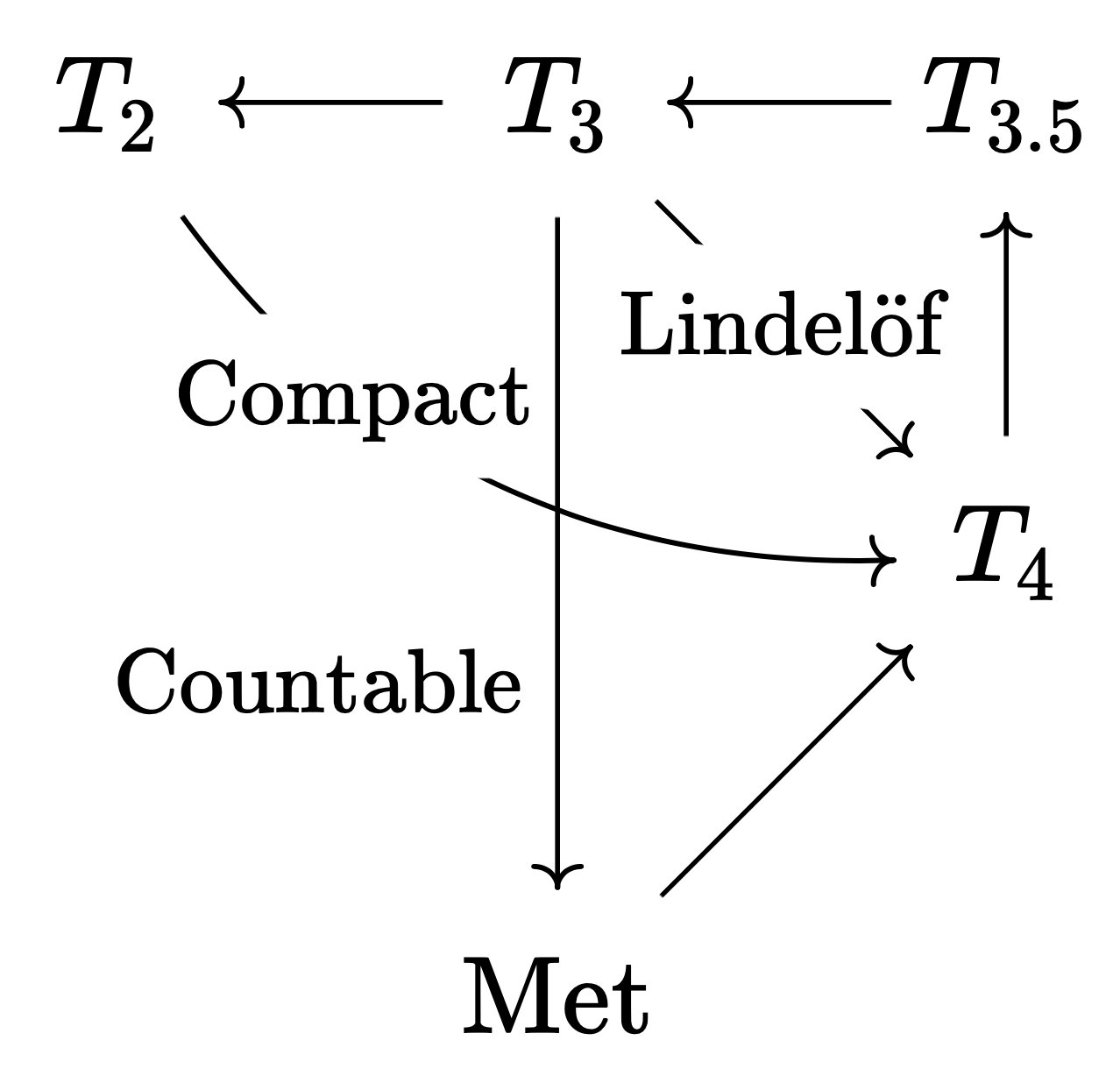
따라서 공간들 간의 시사 관계는 다음과 같다. 화살표의 길이가 길수록 요구되는 조건이 강해진다. $T_2 \to T_4$는 $T_3 \to T_4$보다 엄격히 어려운 시사 관계이며, 이것은 전자에서 요구되는 콤팩트성이 후자에서 요구되는 린델뢰프보다 엄격히 강한 조건인 데에서 드러난다. 마찬가지로 $T_3 \to \mathrm{Met}$는 $T_3 \to T_4$보다 엄격히 어려운 시사 관계이며, 전자에서 요구되는 2차 가산성은 후자에서 요구되는 린델뢰프보다 엄격히 강한 조건이다. 그러나 $T_2 \to T_4$와 $T_3 \to \mathrm{Met}$는 어느 한쪽이 엄격히 어려운 시사 관계가 아니다 (두 화살표의 길이는 엇비슷하다). 이것은 콤팩트성과 2차 가산성이 일반적으로 서로를 시사하지 않는다는 점에서 드러난다.

증명

$X$가 2차 가산인 정규 공간이라고 하자. 다음의 보조정리를 증명한다.

보조정리. $X$를 $[0, 1]$에 사상시키는 연속함수의 가산족 $\mathcal{F}$가 존재하여, 임의의 $x_0 \in X$와 그 근방 $U$에 대해, $f(x_0) > 0$이고 $f[X \setminus U] = \lbrace 0 \rbrace $인 $f \in \mathcal{F}$가 존재한다.

$x_0$와 $U$가 주어졌을 때 그러한 $f$가 존재함은 우리손 보조정리로부터 알 수 있다. 우리가 해야할 일은 이를 가산 함수족으로 줄이는 것이다. $\mathcal{B} = \lbrace B_n \rbrace $이 $X$의 가산인 위상기저라고 하자. $B_m \subset B_n$일 때, 우리손 보조정리로부터 $f_{nm}: X \to [0, 1]$을 다음을 만족하는 연속함수로 정의하자.

• $f_{nm}[\overline{B_m}] = 1$
• $f_{nm}[X \setminus B_n] = 0$

$\mathcal{F} = \lbrace f_{nm} \rbrace $으로 정의하자. 임의의 $x_0$와 그 근방 $U$가 주어졌을 때, 위상기저의 정의에 의해 $x_0 \in B_n \subset U$인 $B_n$이 존재한다. 또한 정규성에 의해 $x \in \overline{V} \subset B_n$인 열린집합 $V$가 존재한다. 다시 위상기저의 정의에 의해 $x \in B_m \subset V$인 $B_m$이 존재한다. 이때 $f_{nm} \in \mathcal{F}$가 보조정리의 조건을 만족하는 함수이다. □

이제 본 정리를 증명하자. 아이디어는 $X$를 $[0, 1]^\omega$에 임베딩하는 것이다. $[0, 1]^\omega$에 곱 위상이 주어지면 거리 공간임이 알려져 있으므로 $X$는 거리 공간의 부분공간과 동형인 공간으로서 거리화 가능함이 보여진다.

$\mathcal{F} = \lbrace f_n \mid n \in \omega \rbrace $가 보조정리로서 주어지는 가산 함수족이라고 하자. 다음과 같이 $F: X \to [0, 1]^\omega$를 정의한다.

\[F: x \mapsto (f_1(x), f_2(x), f_3(x), \dots)\]

$F$가 임베딩을 보이자. 즉, $F$가 연속이고, 단사이며, 정의역과 치역의 동형사상임을 보여야 한다.

각 $f_n$은 연속이므로 곱 위상의 성질(정의이기도 하다)에 의해 $F$는 연속이다. $F$가 단사임은 $X$가 하우스도르프라는 사실에서 따라 나온다. 따라서 다음을 보이면 충분하다.

$U \subset X$가 열린집합일 때, $F[U]$는 $\mathrm{im} F$에서 열린집합이다.

임의의 $y_0 \in F[U]$에 대해 $y_0 \in V \subset F[U]$이며 $\mathrm{im} F$에서 열린 $V$가 존재함을 보이자. $F[U]$의 정의에 의해 어떤 $x_0 \in X$가 존재하여 $F(x_0) = y_0$이다. $x_0$와 $U$에 대해 보조정리를 만족하는 함수가 $f_n \in \mathcal{F}$라고 하자. $f_n(x_0) = 1$이므로 $(y_0)_n = 1$이다. 따라서 $W = \pi_n^{-1}(0, 1] \subset [0, 1]^\omega$와 같이 정의하면 $W$는 $y_0$를 원소로 가지는 $[0, 1]^\omega$에서 열린집합이다.

$W \cap \mathrm{im} F \subset F[U]$임을 보이자. 임의의 $w \in W$는 $F(x_1) = w$와 같이 쓸 수 있다. 추가로 $w \in \mathrm{im} F$라면 $f_n(x_1) = 1$이다. 그런데 $f_n$은 $U$ 외부에서는 $0$이므로, $x_1 \in U$이다. 따라서 $w \in F[U]$이다. 따라서 $W \cap \mathrm{im} F$는 $F[U]$에 포함되며 $y_0$를 원소로 가지는 $\mathrm{im} F$의 열린집합이다. 따라서 $F[U]$는 $\mathrm{im} F$에서 열린집합이다. ■

고찰

• 우리손 거리화 정리는 나가타-스미로느프 거리화 정리_{Nagata-Smirnov metrisation theorem}로 강화할 수 있다. 진술은 다음과 같다.

  $X$가 거리화 가능할 필요충분조건은 $X$가 정칙이며 가산-국소적으로 유한한_{countably locally finite} 위상기저를 가지는 공간인 것이다.

  위상공간 $X$의 부분집합들로 이루어진 집합족 $\mathcal{A}$가 국소적으로 유한하다는 것은, 임의의 $x \in X$에 대해 어떤 근방 $U$가 존재하여 $U$가 $\mathcal{A}$의 오직 유한한 개수의 집합과만 교집합을 가진다는 것이다. 위상기저 $\mathcal{B}$가 가산-국소적으로 유한하다는 것은, 각각의 $\mathcal{B}_n$이 국소적으로 유한이도록 $\mathcal{B} = \bigcup_{n \in \omega}\mathcal{B}_n$와 같이 적을 수 있다는 것이다.

• 우리손 거리화 정리의 증명을 살짝 변형하면 다음 사실을 발견할 수 있다.

  정리. $T_1$ 공간인 $X$에 대해, $\lbrace f_{\alpha} \rbrace _{\alpha \in J} $가 다음 조건을 만족하는 연속함수 $f_\alpha : X \to [0, 1]$의 모임이라고 하자: 임의의 $x_0 \in X$와 근방 $U$에 대해, 어떤 $\alpha \in J$가 존재하여 $f_\alpha(x_0) = 1$이고 $f_\alpha[X \setminus U] = \lbrace 0 \rbrace $이다. 이때, $F(x) = (f_\alpha(x))_{\alpha \in J}$는 $X$를 $[0, 1]^J$로 임베딩하는 사상이다.

  $T_1$ 조건을 생략하면 $F$는 단사가 아닐 수 있음을 확인하라. 위 정리는 스톤-체흐 콤팩트화_{Stone-Čech compactification}를 증명하는 데 사용된다.

The Urysohn Lemma and Urysohn Metrisation Theorem

09 Jul 2025

Urysohn Lemma. Let $X$ be a normal space. If $A$ and $B$ are disjoint closed sets in $X$, then there exists a continuous function $f: X \to [0, 1]$ such that $f[A] = \lbrace 0 \rbrace$ and $f[B] = \lbrace 1 \rbrace$.

The separation axioms, e.g. normality, separate points from closed sets in the given space. The significance of the Urysohn Lemma lies in the fact that, in the case of the normal space, two closed sets can be further separated in a nice space. Specifically, with respect to an appropriate continuous map defined on the normal space to $[0, 1]$, two closed sets can be separated in $[0, 1]$. And the myriad “nice” properties of $[0, 1]$ — being a compact Hausdorff metric space, and a space which we are very familiar with and can visualise easily — suggest the remarkable potential of the Urysohn lemma.

Proof

Let us denote $Q = [0, 1] \cap \mathbb{Q}$ (actually it suffices for $Q$ to be a countable dense subset of $[0, 1]$). Since $Q$ is countable, there exists an enumeration of the elements of $Q$. For instance, consider the lexicographic enumeration of the numerators and denominators, $\prec$.

\[0 \prec 1 \prec 1/2 \prec 1/3 \prec 2/3 \prec 1/4 \prec 1/5 \prec 2/5 \prec \cdots\]

Let us now define the collection $\lbrace U_q \rbrace _{q \in Q}$. First, let $U_1 = X \setminus B$ (since $B$ is a closed set, $U_1$ is an open set). By normality, there exists an open set $U_0$ such that $A \subset U_0$ and $\overline{U_0} \subset U_1$. The remaining $U_q$ are recursively defined in the following manner. For any $p \prec q$,

• If $p < q$, then $\overline{U_p} \subset U_q$.
• If $q < p$, then $\overline{U_q} \subset U_p$.

By normality, these conditions can be satisfied, allowing us to fully define the collection $\lbrace U_q \rbrace _{q \in Q}$.

Now, let us define the function $f: X \to [0, 1]$ as follows.

\[f(x) = \begin{cases} \sup_{<}\{q \in Q : x \notin U_q \} & x \notin U_0 \\ 0 & x \in U_0 \end{cases}\]

The notation $\sup_<$ indicates that we are taking the supremum with respect to $<$ rather than $\prec$. From the definition, it follows that $f[A] = 0$ and $f[B] = 1$.

To complete the proof, we must show that $f$ is continuous. Since $\lbrace B_\epsilon(q) \cap [0, 1] : q \in Q, \epsilon \in \mathbb{Q}_{>0} \rbrace$ forms a basis for the topology on $[0, 1]$, it suffices to show that for any $q \in Q$ and postivie rational $\epsilon$ smaller than a certain supremum, the set $S_{q, \epsilon} = f^{-1}(B_\epsilon(q) \cap [0, 1])$ is an open set. Indeed,

• If $0 < q < 1$, then $S_{q, \epsilon} = (X \setminus \overline{U_{q-\epsilon}}) \cap U_{q + \epsilon}$, which is an open set.
• If $q = 0$, then $S_{0, \epsilon} = U_\epsilon$, which is an open set.
• If $q = 1$, then $S_{1, \epsilon} = X \setminus \overline{U_{1 - \epsilon}}$, which is an open set.

Thus, $f$ is continuous. ■

Remarks

• The converse of the Urysohn lemma trivially holds. That is, for any closed sets $A, B \subset X$, if there exists a continuous function $f: X \to [0, 1]$ that separates $A$ and $B$, then the sets $U = f^{-1}[0, 1/2)$ and $V = f^{-1}(1/2, 1]$ are disjoint open sets that separate $A$ and $B$, implying that $X$ is normal. In simple terms, in normal spaces, the Urysohn separation property and the separation axiom are equivalent.

• This does not hold in regular spaces. Specifically, given any closed set $F$ and point $a$ in a regular space $X$, it is not always the case that there exists a continuous function $f: X \to [0, 1]$ satisfying $f(a) = 0$ and $f[F] = \lbrace 1 \rbrace$. A regular space that is Urysohn separable is called a Tychonoff space or a completely regular space, which is a strictly stronger condition than regularity.

• The reason the proof of the Urysohn Lemma does not go through for regular spaces is that constructing the collection $\lbrace U_q \rbrace $ satisfying $p < q \implies \overline{U_p} \subset U_q$ requires the normality axiom.

Urysohn Metrisation Theorem

As an application of the Urysohn Lemma, let us prove the Urysohn Metrisation Theorem.

Urysohn Metrisation Theorem. A second countable normal space is metrizable.

Recall that a second countable regular space is a normal space. Hence the statement of the above theorem can be strengthened to “A second countable regular space is metrisable.”

Thus, the implications between spaces can be summarised as follows. Note that the longer the arrow, the stronger the required condition. The implication $T_2 \to T_4$ is strictly more difficult than $T_3 \to T_4$, and this is evidenced by the fact that the former requires a condition — compactness — strictly stronger than the latter — Lindelöf. Similarly, $T_3 \to \mathrm{Met}$ is strictly more difficult than $T_3 \to T_4$, as the second countability required in the former is strictly stronger than the Lindelöf property. However, neither $T_2 \to T_4$ nor $T_3 \to \mathrm{Met}$ is strictly more difficult than the other (the lengths of both arrows are similar). This is again evidenced by the fact that compactness and second countability do not generally imply each other.

Proof

Let $X$ be a second countable normal space. We will prove the following lemma.

Lemma. There exists a countable collection of continuous functions $\mathcal{F}$ mapping $X$ to $[0, 1]$ such that for any point $x_0 \in X$ and its neighbourhood $U$, there exists a function $f \in \mathcal{F}$ satisfying $f(x_0) > 0$ and $f[X \setminus U] = \lbrace 0 \rbrace$.

Given $x_0$ and $U$, the existence of such an $f$ follows from the Urysohn Lemma. Our task is to reduce this to a countable collection of functions. Let $\mathcal{B} = \lbrace B_n \rbrace $ be a countable basis for the topology on $X$. When $B_m \subset B_n$, we define a continuous function $f_{nm}: X \to [0, 1]$ satisfying the following conditions according to the Urysohn Lemma:

• $f_{nm}[\overline{B_m}] = 1$
• $f_{nm}[X \setminus B_n] = 0$

Let $\mathcal{F} = \lbrace f_{nm} \rbrace $. Given any point $x_0$ and its neighbourhood $U$, by the definition of a basis, there exists a basis element $B_n$ such that $x_0 \in B_n \subset U$. Furthermore, by normality, there exists an open set $V$ such that $x \in \overline{V} \subset B_n$. Again, by the definition of a basis, there exists a basis element $B_m$ such that $x \in B_m \subset V$. Hence $f_{nm} \in \mathcal{F}$ satisfies the conditions of the lemma. □

Now, let us prove the main theorem. The idea is to embed $X$ into $[0, 1]^\omega$, as $[0, 1]^\omega$ equipped with metric topology is known to be a metric space. It then follows that $X$ is metrisable, being a space homeomorphic to a subspace of a metric space.

Let $\mathcal{F} = \lbrace f_n \mid n \in \omega \rbrace $ be the countable collection of functions given by the lemma. We define the mapping $F: X \to [0, 1]^\omega$ as follows:

\[F: x \mapsto (f_1(x), f_2(x), f_3(x), \dots)\]

We will show that $F$ is an embedding. That is, we need to demonstrate that $F$ is continuous, injective, and a homeomorphism between the domain and the image.

Since each $f_n$ is continuous, by the properties of the product topology, $F$ is continuous (side note: one can regard this as the definition of the product toplogy). The injectivity of $F$ follows from the fact that $X$ is Hausdorff. Therefore, it suffices to show the following:

If $U \subset X$ is an open set, then $F[U]$ is open in $\mathrm{im} F$.

Let us show that for any $y_0 \in F[U]$, there exists a set $V \subset F[U]$ open in $\mathrm{im} F$ that contains $y_0$. By the definition of $F[U]$, there exists some $x_0 \in X$ such that $F(x_0) = y_0$. Let $f_n \in \mathcal{F}$ be a function satisfying the conditions of the lemma for $x_0$ and $U$. Since $f_n(x_0) = 1$, it follows that $(y_0)_n = 1$. Therefore, $W = \pi_n^{-1}(0, 1] \subset [0, 1]^\omega$ is a set containing $y_0$ that is open in $[0, 1]^\omega$.

Now, we need to show that $W \cap \mathrm{im} F \subset F[U]$. For any $w \in W$, we can write $F(x_1) = w$. Additionally, if $w \in \mathrm{im} F$, then $f_n(x_1) = 1$. However, since $f_n$ vanishes outside of $U$, it follows that $x_1 \in U$. Thus, $w \in F[U]$, i.e. $W \cap \mathrm{im} F$ is contained in $F[U]$ and is an open set in $\mathrm{im} F$ containing $y_0$. Hence, $F[U]$ is an open set in $\mathrm{im} F$. ■

Remarks

• The Urysohn Metrisation Theorem can be strengthened to the Nagata-Smirnov Metrisation Theorem. The statement is as follows:

  A space $X$ is metrizable if and only if $X$ is regular and has a countably locally finite topology basis.

  A collection of subsets $\mathcal{A}$ of a topological space $X$ is said to be locally finite if for any point $x \in X$, there exists a neighbourhood $U$ such that $U$ intersects only finitely many sets from $\mathcal{A}$. A topological basis $\mathcal{B}$ is said to be countably locally finite if it can be expressed as $\mathcal{B} = \bigcup_{n \in \omega}\mathcal{B}_n$ where each $\mathcal{B}_n$ is locally finite.

• A slight modification of the proof of the Urysohn Metrisation Theorem leads to the following result.

  Theorem. Let $X$ be a $T_1$ space, and let $\lbrace f_{\alpha} \rbrace_{\alpha \in J}$ be a collection of continuous functions $f_\alpha : X \to [0, 1]$ satisfying the following condition: for any point $x_0 \in X$ and its neighbourhood $U$, there exists $\alpha \in J$ such that $f_\alpha(x_0) = 1$ and $f_\alpha[X \setminus U] = \lbrace 0 \rbrace$. Then, the mapping $F(x) = (f_\alpha(x))_{\alpha \in J}$ embeds $X$ into $[0, 1]^J$.

  Omitting the $T_1$ condition may result in $F$ not being injective. This theorem is used to prove the Stone-Čech compactification.

크립키-비트겐슈타인 역설

03 Jul 2025

“2.2. 성향적 분석” 절에서 크립키의 원 논문과는 독자적인 필자의 보론이 많이 들어갔으니 유의 바랍니다.

개요

크립키는 비트겐슈타인의 ⟪철학적 탐구⟫의 핵심이 소위 규칙 따르기에 대한 회의주의_{Skepticism about rule following}에 있다고 주장한다.

크립키의 독해에 따르면 ⟪탐구⟫의 §1-137은 비트겐슈타인이 ⟪논리철학논고⟫의 언어관을 비판하고 극복하는 대목이다. §138-242에서는 규칙 따르기에 대한 회의주의가 제시된다. “앨리스는 ‘+’로 덧셈을 의미한다”와 같은 명제에 대응되는 사태가 있는지에 관해 의문을 제기하는 회의주의 논증은, ⟪논고⟫의 언어관이 올바를 수 없음을 보이는 최종적인 논증이라는 점에서 §1-137을 확정지을 뿐 아니라, 의미의 문제를 해명하는 이론은 어떠한 형태로든 가능하지 않다는 궤멸적인 결론을 시사하는 듯하다.

크립키에 따르면 비트겐슈타인은 이에 대해 “회의주의적 해답”을 제시한다. 즉, 회의주의자의 결론 — “앨리스는 ‘+’로 덧셈을 의미한다’“에 대응하는 사태는 없다 — 을 받아들이되, 그것이 어떻게 “초록색 생각이 잠을 잔다”와 같은 명제와는 달리 유의미하게 사용될 수 있는지를 해명하는 것이다. 그 해답이란, 언어의 의미는 그것이 공동체에서 가지는 기능과 불가결하며, 따라서 의미에 대한 논의는 개별 언어 사용자 단위에서는 공허하지만 언어 공동체 단위에서는 유효하다는 언어의 공적성을 강조하는 것이다.

§243 이후는 “회의주의적 해답”을 기타 철학적 문제에 적용하는 대목이다. 회의주의적 해답의 함의 중 하나는 사적 언어_{private language}의 불가능성이다. 그럼에도 사적인 방식으로 작동하는 듯한 영역의 언어가 대표적으로 두 가지 있는데, 바로 수학적 언어와 심리적 언어이다. 그러나 비트겐슈타인은 수학적 언어와 심리적 언어가 사적 언어에 해당한다는 생각이 착각이라고 역설한다. 이 대목에서 우리는 비트겐슈타인 특유의 수학철학적 · 심리철학적 입장을 엿볼 수 있다.

1. 크립키-비트겐슈타인 역설

크립키-비트겐슈타인 역설의 결론은 다음과 같다.

“화자 $A$는 기호 $s$로 의미 $m$을 의미한다” 꼴의 명제¹에는 대응되는 사태가 없다. 즉, 해당 명제는 진릿값을 결여한다.

따라서 가령 “앨리스는 ‘+’로 덧셈을 의미한다”라는 명제는 “앨리스의 생각은 초록색이다”라는 명제만큼이나 불가해한 명제이다.

1.1. 회의주의자의 등장

그렇다면 도대체 어째서 크립키-비트겐슈타인은 이토록 극단적인 주장을 하는 것일까? 논증의 핵심은, 언어 사용자가 단어의 의미를 파악하는 과정에 숨은, 간과하기 쉽지만 실로 모순적인 측면에 있다. 바로 과거의 유한한 학습 경험으로부터, 해당 단어가 사용될 수 있는 무한한 사례들에 대해 올바른 추론을 할 수 있어야 한다는 것이다.

예를 들어 앨리스는 지금까지 50이 넘는 두 수의 덧셈을 해본 적이 없다고 하자. 그렇다고 해도 누군가 앨리스에게 ’68 + 57’을 묻는다면 그는 어렵지 않게 ‘125’라고 답할 것이다. 그런데 이때 앨리스에게 한 회의주의자가 다가오더니, ‘125’라는 그의 답은 틀렸으며, 앨리스가 내놓았어야 하는 답은 ‘5’였다고 주장한다. 구체적으로, 회의주의자는 다음을 주장한다.

만약 앨리스가 과거에 ‘+’에 부여하던 의미와 현재 ‘+’에 부여하는 의미가 일치한다면, 앨리스는 ‘5’라고 답했어야 한다.

왜냐하면 — 적어도 회의주의자에 따르면 — 앨리스가 과거에 ‘+’에 부여했던 의미는 사실 덧셈(+)이 아니라 컷셈(⨁)이었기 때문이다. 컷셈의 정의는 다음과 같다.

\[x \oplus y = \begin{cases} x + y & x, y < 50 \\\ 5 & \text{otherwise} \end{cases}\]

이에 앨리스는 과거부터 자신은 ‘+’를 컷셈이 아닌 덧셈의 의미를 사용했다고 즉각 반박할 것이다. 그런데 여기부터 본격적인 문제가 시작된다. 과거에 앨리스가 ‘+’에 부여한 의미가 컷셈이 아닌 덧셈이었음을 어떻게 입증할 수 있는가? 문제의 가정으로 인해, 과거에 앨리스가 수행한 ‘+’의 계산 기록들로부터 이를 입증하는 것은 불가능하다.

방금 등장한 ‘입증’이라는 표현으로 인해 이 문제가 인식론에 속하는 것처럼 보일 수 있다 (“우리는 앨리스가 ‘+’로 덧셈을 의미한다는 사실을 어떻게 알 수 있을까?”). 그러나 크립키가 묻는 것은, 앨리스의 머리 속까지 들여다 볼 수 있는 전지전능한 관찰자라고 할지라도 앨리스가 ‘+’로 덧셈을 의미하는지, 혹은 덧셈과 충분히 많은 경우에 일치하는 비표준적인 연산을 의미하는지 알 수 있는가이다. 이런 점에서 크립키가 제시하는 회의주의는 존재론적인 것이다. 문제의 요점은 “앨리스가 컷셈이 아닌 덧셈을 의미한다”에 대응하는 사태_case가 있는가이다. 이는 후술하다시피 크립키가 반사실적 조건문 혹은 가능세계를 통해 회의주의를 해소하려는 시도까지 검토한다는 점에서 — 비록 그 시도 또한 실패한다고 결론 내리지만 — 드러난다.

1.2. 두 가지 조건

회의주의자의 주장에는 두 가지 주목할 점이 있다. 첫째, 회의주의자의 주장은 가정문이다. 회의주의자는 앨리스가 어떤 경우에서든 ’5’라고 답해야 함을 주장하는 것이 아니다. 그가 주장하는 바는, 만약 앨리스가 과거에 ‘+’에 부여하던 의미와 현재 ‘+’에 부여하는 의미가 일치한다면 ’5’라고 답해야 한다는 것이다. 둘째, 회의주의자의 주장은 규범적이다. 회의주의자의 주장은 — 앞서 말한 조건이 만족되었을 때 — 앨리스는 ‘5’라고 답할 것이라는 주장이 아니라 ‘5’라고 답해야 한다는 주장이다.² 달리 말해, 회의주의자는 만약 앨리스가 ’68 + 57’에 대해 ‘5’라고 대답했더라면 그 대답은 정당했을 것 임을 주장한다.

따라서 회의주의자의 주장에 대한 반박 또한 두 가지 특징을 갖춰야 한다. 첫째, 화자에 관한 어떠한 사실이, 해당 화자가 특정 기호를 특정 의미로 사용함을 구성하는지 설명해야 한다. 이 설명은 회의주의자의 주장에서 가정이 무엇을 의미하는지를 해명하기 위해 필요하다.³ 둘째, 해당 사실이 어떠한 방식으로 화자의 언어 사용을 정당화하는지 설명해야 한다. 이 설명은 회의주의자의 결론이 규범적이기 때문에 필요하다.

두 번째 조건의 의의가 안 와닿을 수도 있기 때문에 조금 더 설명을 해 보겠다. 가령 어떤 매드사이언티스트가 오더니 회의주의자에게 이렇게 말했다고 하자.

사실 나는 과거에 앨리스를 원자 단위로 스캔한 적이 있다. 그래서 나는 너의 말을 듣고 그 스캔본을 본따 만든 앨리스-2에게 ’68 + 57‘을 물어보았고, 앨리스-2는 ’125‘라고 대답했다. 따라서 과거의 앨리스는 ’+‘로 컷셈을 의미하지 않았다.

그러나 매드사이언티스트의 실험은 회의주의자의 주장을 반박하는 데 역부족이다. 매드사이언티스트의 실험은 두 번째 조건을 만족하지 않기 때문이다. 해당 실험의 결과는 앨리스가 언제나 ‘125’라고 답했을 것임을 보증할 뿐, 앨리스가 언제나 ‘125’라고 답해야만 했음은 보증하지 않는다.

이는 체계적 계산 오류의 사례를 통해 더 명확히 이해할 수 있다. 가령 덧셈을 처음 배우는 아이는 종종 받아올림을 까먹곤 한다. 그런 아이는 ’68 + 57’에 대해 ‘125’가 아니라 ‘115’라고 대답할 것이다. 그런데 모종의 문제로 인해 어른이 될 때까지 받아올림 실수를 교정하지 못한 존슨이라는 사람이 있다고 하자. 존슨은 덧셈이 무엇인지 이해하며, 구체적인 덧셈 문제가 아니라 덧셈에 대한 성질을 질문 받으면 — 가령, “결합법칙을 만족하는가?” — 올바르게 대답한다. 다만, 존슨은 그의 실수를 교정해 줄 지도자가 없는 상황에서 ’68 + 57’을 질문 받으면 언제나 ‘115’라고 대답했을 것이며, 앞으로도 그럴 것이다. 이를 두고 우리는 존슨이 ‘+’에 덧셈의 의미를 부여하고 있으나, 그 의미에 정당한 방식대로 ’68 + 57’에 대답하지 못하는 것이라 주장하고 싶다. 바로 이 주장을 성립시키기 위해 두 번째 조건이 필요한 것이다. 두 번째 조건을 만족하지 못하는 의미론을 채택한다면, 우리는 존슨이 ‘+’에 텃셈 — 두 수의 덧셈을 받아올림을 제하고 수행하는 연산 — 혹은 펏셈 — 곁에 지도자가 없는 상황에서는 텃셈을 수행하고, 있는 상황에서는 지도자의 교정을 받아 덧셈을 수행하는 연산 — 의 의미를 부여하고 있다고 수긍해야 하기 때문이다.⁴

2. 회의주의에 대한 반박 검토

2.1. 언어적 해명

회의주의자의 주장을 들은 앨리스가 내놓을 첫 번째 대답은 아마 이러할 것이다. “과거의 나는 ‘x + y’에 x개의 대상과 y개의 대상을 한데 모아 세는 연산의 의미를 부여해 왔다. 따라서 과거의 나는 ‘+’를 컷셈의 의미로 사용하지 않았다.”

그러나 회의주의자는 이에 대해 또 한번 회의주의를 펼칠 수 있다. 요컨대 그는 과거에 앨리스는 ‘모아 세다’라는 단어를 줄곧 셈_count이 아닌 켐_quont으로 이해하고 있었다고 주장할 수 있다. 묶음을 켄다는 것은 묶음의 크기가 50 미만일 때는 세는 것이고 50을 초과할 때는 5라고 대답하는 것이다.

요지는, ‘+’에 부여한 의미가 무엇인지를 다른 언어적 증거를 통해 입증하려는 시도는 해당 증거 또한 비표준적인 의미가 부여되었을 가능성을 제거하지 못하므로 무한 퇴행에 빠진다는 것이다.⁵

2.2. 성향적 분석_{dispositional analysis}

심리철학에서 성향적 분석은 행동주의_behaviourism가 심리 상태를 설명하는 방식으로, 핵심은 다음과 같다.

심리 상태의 성향적 분석. 주체 $A$가 과거, 현재, 또는 미래에 심리 상태 $\mathfrak{m}$에 있다는 것은, $A$에게 특정 자극 $s$이 주어졌더라면 / 주어진다면 / 주어지게 된다면, $A$는 반응 $b = f_\mathfrak{m}(s)$를 보였을 / 보일 / 보이게 될 것이라는 말이다. 즉, 심리 상태($\mathfrak{m}$)은 자극-반응 대응($f_\mathfrak{m}$)으로 환원된다.

예를 들어 금방 선잠에서 깬 앨리스가, 어둑어둑한 방과 창밖으로 들리는 물방울 소리를 듣고, “지금 비가 오고 있다”라는 믿음을 형성했다고 해보자. 성향적 분석에 따르면 “앨리스는 ‘지금 비가 오고 있다’고 믿는다”의 의미는 다음의 (무수히 많은) 자극-반응 대응과 다름이 없다.

• 친구에게서 같이 밥 먹으러 가자는 전화가 온다면, -> 우산을 챙길 것이다.
• 이웃에게서 밖에 당신의 빨래가 걸려 있다는 연락이 온다면, -> 빨래를 급히 거두러 갈 것이다.
• 내일 야외 일정이 잡힌다면, -> 내일의 날씨를 확인할 것이다, 등등…

만약 이러한 자극-반응 대응에서 크게 어긋나는 현상이 관측된다면 성향적 분석주의자는 앨리스의 믿음에 대한 견해를 수정할 것이다. 예를 들어 앨리스가 외출을 나서는데 우산을 챙기는 대신 선글라스를 챙긴다면, 그는 앨리스가 “비가 오고 있다”는 믿음이 아닌 “햇살이 쨍쨍하다”는 믿음을 가지고 있다고 판단할 것이다.

지금까지의 설명에서 주목할 성향적 분석의 특징은 두 가지이다.

1. 반사실적 조건문을 사용한다. 앨리스가 과거, 현재, 또는 미래에 외출을 나가지 않는다고 하더라도, “앨리스가 외출을 나갔더라면 / 나간다면 / 나가게 된다면 그는 우산을 챙겼을 / 챙길 / 챙기게 될 것이다”는 그가 가졌던 / 가지고 있는 / 가지게 될 믿음에 대한 성향적 분석의 일부를 이룬다.
2. 기술적이다. 성향적 분석은 행동주의를 기반으로 하기 때문에 “앨리스가 외출을 나간다면 그는 우산을 챙겨야 한다” 와 같은 규범적 명제가 아닌, “앨리스가 외출을 나간다면 그는 우산을 챙길 것이다” 와 같은 기술적 명제로 이루어진다. 성향적 분석에 따르면, 만약 앨리스가 외출을 나서는데 우산을 챙기는 대신 선글라스를 챙긴다면, 앨리스는 비가 오고 있다는 믿음을 가지고 있음에도 그에 정당하게 행동하지 않는 것이 아니라, 애초에 비가 오고 있다는 믿음을 가지고 있지 않은 것이다.

크립키는 자신과 사적인 자리에서 규칙 따르기 역설을 논의했던 일부 철학자들이, 성향적 분석의 1번 특징에 의존함으로써 성향적 분석을 통한 역설의 해결을 시도했다고 전한다. 이 접근법은 다음을 주장한다.

의미에 대한 성향적 분석. 화자 $A$가 과거, 현재, 또는 미래에 기호 $s$로 의미 $\mathfrak{m}$을 의미한다는 것은, $s$가 포함된 문장 $\phi$가 $A$에게 주어졌더라면 / 주어진다면 / 주어지게 된다면, $A$는 문장 $\psi = f_\mathfrak{m}(\phi)$로 대답했을 / 대답할 / 대답하게 될 것이라는 말이다. 즉, 의미($\mathfrak{m}$)는 문답 대응($f_\mathfrak{m}$)으로 환원된다.

이 분석에 따르면, 앨리스가 과거, 현재, 또는 미래에 ‘+’로 덧셈을 의미한다는 것은, 앨리스에게 x + y를 물어보았더라면 / 물어본다면 / 물어보게 될 때, $A$는 x와 y의 합으로 대답했을 / 대답할 / 대답하게 될 것이라는 말이다. 이러한 반사실적 조건문을 통해 회의주의를 극복하려는 철학자의 사고 흐름은 대략 다음과 같을 것이다.

1. 회의주의자는 과거의 앨리스가 ‘+’로 덧셈을 의미했는지, 덧셈이 아니지만 충분히 많은 경우에 덧셈과 일치하는 비표준적 연산을 의미했는지 구별하는 사태가 지금까지 없었고, 앞으로도 없을 것임을 지적한다.
2. 1이 주장 가능한 이유는, 앨리스가 지금까지 수행했고, 앞으로 수행할 ‘+’의 연산 횟수가 유한하기 때문이다.
3. 그러나 “과거의 앨리스에게 ’x + y’을 물어보았더라면 나는 x와 y의 합을 대답했을 것이다”, 또는 “미래의 앨리스에게 ‘x + y’를 물어본다면 나는 x와 y의 합을 대답할 것이다”라는 반사실적 조건문을 사용하면, 우리는 2의 유한성을 극복할 수 있다.
4. 이에 따라, 반사실적 조건문은 객관적인 진릿값을 가진다는 사실을 — 가능세계 존재론 등을 통해 — 인정한다면, ”앨리스가 ’+‘로 덧셈을 의미한다“에 대응되는 의미에 대한 성향적 분석은 앨리스가 ‘+’로서 의미하는 연산을 객관적으로 결정한다.

이 논증은 회의주의자에 대한 반박이 갖춰야 할 첫째 조건 — 화자에 관한 어떠한 사실이 해당 화자가 특정 기호를 특정 의미로 사용함을 구성하는지 설명해야 한다 — 을 만족한다. 그 사실이라 함은 반사실적 조건문인 것이다. 그러나 크립키는 둘째 조건 — 해당 사실이 어떠한 방식으로 화자의 언어 사용을 정당화하는지 설명해야 한다 — 을 갖추지 못하므로 성향적 분석은 역설을 해소하는 데 불충분하다고 지적한다. 이는 앞서 지적했듯이 성향적 분석이 본질적으로 기술적이기 때문이다. 크립키의 말을 인용하자면,

좋다. 나는 ‘125’가 내가 주어진 수식에 대해 내놓을 대답임을 알며, (실제로 그렇게 대답하고 있지 않은가!) 어쩌면 — 그저 하나의 주어진 사실로서 — 과거의 나에게 같은 수식이 주어졌다고 하더라도 똑같이 대답했으리라는 사실 또한 안다고 하자. 이 모든 사실들이 도대체 어떻게 — 현재 또는 과거에서 — ‘125’가, 내 내면의 어떤 규칙에 의거하여 도출된 정당화된 답이지, 그저 눈 가리고 아웅하며 내놓은 아무 근거 없는 답이 아니라는 사실을 보여주는가?

Well and good, I know that ‘125’ is the response I am disposed to give (I am actually giving it!), and maybe it is helpful to be told — as a matter of brute fact — that I would have given the same response in the past. How does any of this indicate that — now or in the past — ‘125’ was an answer justified in terms of instructions I gave myself, rather than a mere jack-in-the-box unjustified and arbitrary response?

(이탤릭체는 원문, 강조는 필자)

크립키가 지적하는 바는 다음과 같이 차근차근 이해할 수 있다. 기억을 되살려 보면, 회의주의자에게 대항하는 주장은 다음의 형식을 갖춰야 한다.

주장 1. 만약 앨리스가 과거에 ‘+’에 부여하던 의미와 현재 ‘+’에 부여하는 의미가 일치한다면,

1. 앨리스는 ‘5’라고 답해야 하는 것이 아니라,
2. 앨리스는 ‘125’라고 답해야 한다.

성향적 분석에 의하면 위 주장은 다음과 동의적이다.

주장 1.1. 만약 ‘+’에 대한 과거 앨리스의 문답 성향이 ‘+’에 대한 현재 앨리스의 문답 성향과 일치한다면,

1. 앨리스는 ‘5’라고 답해야 하는 것이 아니라,
2. 앨리스는 ‘125’라고 답해야 한다.

“그저 하나의 주어진 사실로서”, ‘+’에 대한 과거 앨리스의 문답 성향이 두 수가 주어졌을 때 그 합을 말하는 것이었다고 하자. 이 사실을 위에 대입하면,

주장 1.2. 만약 ‘+’에 대한 현재 앨리스의 문답 성향이 두 수가 주어졌을 때 그 합을 말하는 것이라면,

1. 앨리스는 ‘5’라고 답해야 하는 것이 아니라,
2. 앨리스는 ‘125’라고 답해야 한다.

그러나 주장 1을 주장 1.2.로 재진술하였다고 한들, 이를 성립시킬 근거는 여전히 전무하다. 만약 1, 2의 술어부가 “답할 것이다”였다면 주장이 성립하겠지만, 요구된 것은 “답해야 한다”이다. 이것은 문답 성향만 가지고서 알 수 있는 사실이 아니다.

그렇다면 처음부터 1, 2의 술어부를 ”답할 것이다“라고 둘 수는 없을까? 요컨대 회의주의자에게 다음을 주장하는 것이다.

주장 2. 만약 앨리스가 과거에 ‘+’에 부여하던 의미와 현재 ‘+’에 부여하는 의미가 일치한다면,

1. 앨리스는 ‘5’라고 답할 것이 아니라,
2. 앨리스는 ‘125’라고 답할 것이다.

그럴 수는 없다. 앞서 “체계적 계산 오류의 사례”에서 자세히 설명했듯이, 앨리스가 ‘68 + 57’에 대해 ‘125’라고 대답하지 않았다고 해서 그 사실이 즉시 앨리스가 ‘+’로 덧셈을 의미하지 않았음을 시사하지는 않기 때문이다. 우리는 덧셈을 수행함에 있어 때때로 실수를 하곤 하지만, 그런 실수가 저지를 때마다 ’+‘를 덧셈이 아닌 다른 의미로 사용했음을 뜻하지는 않는다. 오히려 내가 ‘+’ 연산을 수행함에 있어 실수를 저지를 수 있다는 사실 자체가, 내가 내놓는 계산 결과가 내가 ‘+’에 부여하는 의미를 결정하는 것이 아니라, 역으로 내가 ‘+’에 부여하는 의미가 선행하여 내가 내놓아야 할 결과를 결정함을 시사한다.

그럼에도 성향적 분석으로 의미의 규범성을 설명하기 위해서는 다음과 같이 회의주의자의 도전을 재해석해야만 할 듯하다.

주장 3. 만약 앨리스가 과거에 ‘+’에 부여하던 의미와 현재 ‘+’에 부여하는 의미를 일치시키고자 한다면,

1. 앨리스는 ‘5’라고 답해야 하는 것이 아니라,
2. 앨리스는 ‘125’라고 답해야 한다.

이는 다음 진술로 이어진다.

주장 3.1. 만약 ‘+’에 대한 현재 앨리스의 문답 성향이 두 수가 주어졌을 때 그 합을 말하는 것이 되고자 한다면,

1. 앨리스는 ‘5’라고 답해야 하는 것이 아니라,
2. 앨리스는 ‘125’라고 답해야 한다.

확실히 주장 3.1은 주장 1.1, 1.2보다는 그럴듯해 보인다. 그러나 필자가 보기에 주장 3.1에도 여전히 문제가 있다.

첫째 문제는, 설령 주장 3이 성립한다고 하더라도 그것이 주장 1을 시사하지는 않는다는 문제이다. $p, q$를 다음과 같이 두자.

• $p:$ 앨리스가 과거에 ‘+‘에 부여하던 의미와 현재 ’+‘에 부여하는 의미가 일치한다.
• $q:$ 앨리스는 ‘125’라고 답한다.

이 경우 주장 1과 주장 3은 각각 다음과 같다. ($W$는 ”하고자 한다“를, $\Box$는 “해야 한다”를 의미)

• 주장 1. $p \rightarrow \Box q$
• 주장 3. $Wp \rightarrow \Box q$

그러나 $p$는 $Wp$를 시사하지 않고 (내가 원하지 않는 일이 나에게 일어날 수 있다) $Wp$ 또한 $p$를 시사하지 않기 때문에 (내가 원하는 일이 나에게 일어나지 않을 수 있다) 주장 1과 주장 3에는 어떠한 논리적 관계도 없다. 구체적으로 전자의 경우로는, ‘+’를 곱셈의 의미로 사용하겠다고 다짐한 반항아 학생이 자신의 다짐이 무색하게 습관적으로 ‘68 + 57‘에 ’125‘라고 대답해버리는 상황이 있다. 후자의 경우로는 ‘+’ 기호를 덧셈의 의미로 사용하고자 하지만 아직 덧셈의 개념을 완전히 숙지하지 못한 학생의 경우가 있다.

둘째 문제는, 애초에 주장 3은 무한 회귀에 빠진다는 것이다. 잠시 설명의 편의를 위해 심리 상태의 사례로 돌아가 보자. 현재의 문제를 심리 상태에 관한 것으로 전환하면 다음과 같을 것이다. 앨리스는 지금 밖에 비가 오고 있다는 믿음을 가지고 있음에도 불구하고 우산이 아닌 다른 물건을 챙긴 채 밖으로 나갈 수 있다. 가령 앨리스가 허겁지겁 외출 준비를 하고는 우산꽂이에서 아무거나 뽑은 채 집을 나섰는데, 손에 잡힌 게 우산이 아니라 지팡이였던 상황을 고려해 보자. 기존의 성향적 분석에 따르면 이 경우 앨리스는 애초부터 비가 오고 있다는 믿음을 가지고 있지 않던 것인데 이는 반직관적인 결론이다. 이에 대해 성향적 분석주의자는 다음의 주장들을 대신 내세울지 모른다.

주장 4. 만약 앨리스가 과거에 ‘어두컴컴한 방과 창밖으로 떨어지는 물방울 소리’에 형성하던 믿음과 현재 동 상황에 형성하는 믿음을 일치시키고자 한다면,

1. 앨리스는 지팡이를 챙겨야 하는 것이 아니라,
2. 앨리스는 우산을 챙겨야 한다.

주장 4.1. 만약 ‘어두컴컴한 방과 창밖으로 떨어지는 물방울 소리’에 대해 앨리스가 보였을 자극-반응 대응과, 동 상황에 대한 현재 앨리스의 자극-반응 대응을 일치시키고자 한다면,

1. 앨리스는 지팡이를 챙기는 것이 아니라,
2. 앨리스는 우산을 챙겨야 한다.

주장 4.2. 만약 ‘어두컴컴한 방과 창밖으로 떨어지는 물방울 소리’에 대한 앨리스의 자극-반응 대응이 외출을 나가는 상황에 대하여 우산을 챙기는 것이 되고자 한다면,

1. 앨리스는 지팡이를 챙기는 것이 아니라,
2. 앨리스는 우산을 챙겨야 한다.

이미 앞서 말했듯이 주장 4는 $Wp \rightarrow \Box q$의 형태이므로 애초에 $p \rightarrow \Box q$와 논리적 관계가 없지만, 그 문제를 차치하더라도 일면 타당해 보이는 주장 4.2에는 본질적인 문제가 있다. 애당초 우리가 성향적 분석을 시도하는 이유는 심리 상태에 관한 진술을 행동주의적인 표현으로 옮기기 위해서이다. 그런데 주장 4.2는 한 특정 심리 상태 — 밖에 비가 오고 있다는 믿음 — 에 관한 진술을, 다른 심리 상태 — 외출을 나가는 상황에 대하여 우산을 챙기는 반응을 보이고자 하는 의도 — 에 관한 진술로 바꾼 것에 지나지 않는다. 이제 우리는 누군가가 ‘외출을 나가는 상황에 대하여 우산을 챙기는 반응을 보이고자 하는 상태’가 무엇인지를 성향적 분석으로 설명해야 하는데, 이는 결국 무한 회귀에 빠지는 것이다.

동일한 이유로 주장 3 또한 무한회귀에 빠진다. 앞선 논의를 되새겨 보면, 회의주의자의 주장에 대한 반박이 갖춰야 할 필요조건 중 하나는 “화자에 관한 어떠한 사실이, 해당 화자가 특정 기호를 특정 의미로 사용함을 구성하는지 설명할 것“이다. 그런데 주장 3.1은 이 문제에 대해 “문답 성향을 특정한 방식에 일치시키고자 하는 의도”라는 답을 제시한다. 그렇다면 회의주의자는 이에 대해, ”화자에 관한 어떠한 사실이, 해당 화자가 ‘+’ 기호에 대한 문답 성향을 특정한 방식 — 이를테면, 컷셈이 아닌 덧셈에 대응되는 문답 성향 — 에 일치시키고자 하는 의도를 가지고 있음을 구성하는가?“ 라고 반문할 수 있다.

결론적으로, 성향적 분석으로 의미의 문제를 해결하려는 시도는 의미의 규범성을 설명하지 못한다. 규범성을 설명할 수 있도록 성향적 분석을 억지로 끼워맞추려는 시도는 문제가 요구하는 바를 벗어날 뿐 아니라, 무한 회귀의 오류에까지 빠지게 된다.

2.3. 기계주의

그렇다면 언어적 해명이나 성향적 분석과 같은 추상적인 설명에 급급하는 대신, 아예 ‘+’가 의미하는 연산에 대응되는 구체적인 기계를 설계해 제시해 줌으로써 회의주의자에게 대응할 수는 없을까? 가령 기계식 계산기를 제작하거나, 논리 회로로 전가산기를 설계해 보이는 것이다. 그러나 크립키는 이 시도 또한 크게 세 가지 이유에서 부적절한다고 주장한다.

첫째, 기계의 사용법이 여전히 해명을 요하는 문제로 남는다. 튜링 기계로 예를 들면, 우리는 튜링 기계가 출력하는 이진 나열을 이진법으로 해석하여 결과를 읽을 것이다. 그러나 회의주의자는 이 기계를 해석하는 올바른 방식이 퀴진법 이며, 퀴진법에 따르면 튜링 기계는 덧셈이 아니라 컷셈을 출력하고 있다고 주장할 수 있다.

둘째, 실제 기계는 오직 유한한 입력만을 받을 수 있다. 그런 의미에서 실제 기계는 앨리스보다 더 ‘유능한’ 존재가 되지 못한다. 그렇다고 실제 기계를 구현하는 대신 기계의 알고리즘을 제시한다면, 이는 다시 “2.1. 언어적 해명”으로 돌아가는 것이다.

셋째, 기계는 오작동할 수 있다. 누군가 기계를 떨어뜨려서 기어가 빠지거나, 너무 오래 쓰다 보니 전선이 녹을 수도 있다. 따라서 우리는 기계에게 의미 해명의 책임을 전임하여 “이 기계는 언제나 내가 의미하는 연산을 계신한다”라고 주장할 수 없다. 그렇다고 우리는 “이 기계는 오작동하지 않는 한 언제나 내가 의미하는 연산을 계산한다”라고 주장할 수도 없다. 그렇게 주장하기 위해서는 기계가 정상적으로 작동하고 있는지 오작동하는지 판단하는 기준을 제시해야 하는데, 그 기준은 결국 우리가 이 기계를 어떤 의도로 사용하고자 하는지에 달려 있을 것이다 (어떤 괴이한 설계자는 기어의 빠짐과 전선의 녹아내림을 통해 덧셈을 계산하는 기계를 만들 수도 있지 않은가?). 따라서 오작동하지 않는 한 이라는 표현을 사용하는 순간 기계가 아닌 화자의 의도가 선행하게 된다.

2.4. 오컴의 면도날

크립키는 다음의 주장도 고려한다.

오캄 의미론. 두 가설 “화자 $A$는 기호 $s$로 의미 $\mathfrak{m}_1$을 의미한다”와 “화자 $A$는 기호 $s$로 의미 $\mathfrak{m}_2$를 의미한다”가 비결정 상태에 있을 때, $\mathfrak{m}_1$과 $\mathfrak{m}_2$ 중 더 단순한 쪽의 가설을 우선적으로 받아들여야 한다.

예를 들어 다음 두 가설을 보자.

    H1. 과거에 앨리스는 ‘+’로 덧셈을 의미했다.

    H2. 과거에 앨리스는 ‘+’로 컷셈을 의미했다.

과거에 앨리스가 수행한 ‘+’ 연산 기록의 양항은 모두 50 이하이므로, H1과 H2는 비결정 상태에 있다. 오캄 의미론이 주장하는 바는 이 경우 우리는 H1설을 우선적으로 받아들여야 한다는 것이다. 덧셈이 컷셈보다 더 단순한 연산이기 때문이다.

그러나 크립키는 이 주장을 짧게만 언급하고 넘어가는데, 회의주의를 논박하는 데 있어 부적절하다는 사실이 자명하기 때문이다. 이는 ‘단순하다’라는 술어가 주관적이라든가, 정의하기 어렵다든가, 화성인에게는 컷셈이 덧셈보다 더 단순할지도 모른다 등의 이유 — 물론 이 이유들도 매우 정당하다 — 때문만이 아니다. 더 본질적인 이유는, 회의주의 논증의 결론이 “H1과 H2 중 어느 하나가 참인지 미정이다”가 아니라, “H1과 H2 중 어느 하나가 참이라는 사실이 어떤 사태에 해당하는지가 미정이다”라는 것이다. 회의주의 논증에 따르면 우리는 H1과 H2가 서로 다른 사태를 나타내는지도 확실하지 않은 상황이다. 이토록 가설이 나타내는 사태가 명확하지 않다면 우리는 오컴의 면도날의 적용이 정당한지를 따지기도 전에 애초에 적용할 수 없다.

2.5. 심리주의

크립키가 더 중요하게 고려하는 반론은 심리주의이다.

심리주의 의미론. 화자 $A$가 기호 $s$로 $\mathfrak{m}$을 의미한다는 것은, 화자의 내면에 $\mathfrak{m}$에 대응되는 특유한_queer 심리적 경험 $p_\mathfrak{m}$이 형성되었다는 말이다.

여기서 “특유한 심리적 경험”은 퀄리아와 비슷한 것으로 생각할 수 있다. 요컨대 “빨간색을 보는 것”이 다른 술어나 경험으로 환원될 수 없는 특유 경험이듯이, “‘+’로 덧셈을 의미하는 것” 또한 그러한 특유 경험이라는 것이다.

크립키는 그러한 특유 경험이 존재할 가능성을 부정하지 않는다.⁶ 그러나 크립키는 심리주의 의미론 또한 회의주의 논증을 해결하지 못함을 지적한다. 문제는 어김없이 “1.2. 두 가지 조건” 중 2번 조건에 있다.

단적인 예시로, 앨리스는 ‘+’ 기호를 사용할 때마다 이마에서 통증을 느낀다고 해보자. 이 사실은 “1.2. 두 가지 조건” 중 1번 조건을 만족한다. 즉, 앨리스가 과거에 ‘+’에 부여한 의미와 현재 부여하는 의미가 같다는 것은 앨리스가 ‘+’ 기호를 사용할 때 느낀 과거의 통증과 현재의 통증이 질적으로 같다는 것이다. 그러나 그렇다고 해서, 그 통증이 도대체 어떤 방식으로 앨리스에게 ’68 + 57’에 대해 ‘125’라고 대답해야 한다는 사실을 알려줄 수 있다는 말인가?

크립키는 이 논의를 보다 일반적인 경험주의 반박과 연관짓는다. 경험주의에 따르면 내가 ‘삼각형’을 의미한다는 것은 내가 내면에서 삼각형의 인상을 떠올린다는 것이다. 그런데 이 삼각형의 인상이 어떻게 내가 ‘삼각형’이라는 단어를 사용하는 규칙을 알려준다는 말인가? 가령 나의 머리에 떠오른 인상이 예각삼각형이라고 하더라도 나는 둔각삼각형을 가리키며 정당하게 삼각형이라고 말할 수 있다. 반면 나의 머리에 떠오른 인상과 정확히 같은 모양의 밑변을 가지는 삼각뿔을 가리키며 삼각형이라고 말할 수는 없다. 요컨대 머리 속에서 어떤 인상이 제시된다고 한들, 그 인상을 어떻게 해석해 내야 할지는 미궁에 쌓여있다.

그럼에도 크립키는 우리가 반대 극단으로 치우쳐, 심리적 경험 내지 느낌이 의미의 문제와 완전히 무관하다고 결론내려서는 안 됨을 강조한다. 크립키는 ⟪철학적 탐구⟫의 논의에서 파생되는 다음의 사례들을 거론한다.

• 같은 단어를 수십 번 말하다 보면 마치 단어에서 의미가 빠져나가고 껍질만 남은 것처럼 ‘낯설게’ 느껴지는 현상
• ’배’를 운송수단을 떠올리며 말할 때와 과일을 떠올리며 말할 때의 차이 (이것을 네커 큐브 착시와 비교해 보라)
• 심리철학의 철학적 좀비와 유사한, 의미론적 좀비 — 발화 기록만으로는 일반적인 언어 사용자와 구별되지 않으나 내면에 어떠한 의미론도 가지고 있지 않은 화자

크립키는 위 사례들이 해명되어야 할 문제임을 인정하지만, 안타깝게도 지면의 문제로 인해 넘어간다.

2.6. 플라톤주의

마지막으로 크립키가 고려하는 반론은 플라톤주의다.

플라톤주의 의미론. 화자 $A$가 기호 $s$로 $\mathfrak{m}$을 의미한다는 것은, 화자가 의미 $\mathfrak{m}$에 대응되는 플라톤적 대상 $\pi_\mathfrak{m}$을 지향한다는 것이다.

따라서 앨리스가 ‘+’로 덧셈을 의미한다는 것은, 앨리스가 플라톤적 덧셈과 모종의 관계를 맺는 것이다.

이것은 프레게가 회의주의자에게 제시했을 대답이었을 걸로 짐작할 수 있다. 프레게에 따르면 기호는 화제에게 특정한 뜻_{sense, Sinn}으로서 나타나는데, 뜻은 지시체를 유일하게 결정한다. 여기서 뜻과 지시체는 플라톤적 대상이다.

프레게의 언어철학: 기호 -> 화자 -> 뜻 -> 지시체

그러나 크립키는 플라톤주의 또한 이전과 거의 같은 논리로 기각한다. 플라톤주의는 유한한 인간이 어떻게 덧셈과 같은 무한집합과 관계 맺을 수 있는지를 설명하지 못할 뿐더러, 이에 따라 앨리스가 지향하는 플라톤적 대상이 덧셈 집합인지 컷셈 집합인지를 어떻게 결정하냐는 문제를 낳는다.

이상으로 크립키-비트겐슈타인 역설과, 이에 대한 주요 반박 및 재반박을 살펴 보았다. 최종적으로 크립키는 회의주의 논증에 대한 직설적인 반박은 불가능하다고 결론 내린다. 따라서 이제 논의는, 정말로 회의주의 논증의 결론대로 “앨리스는 ‘+’로 덧셈을 의미한다”가 “앨리스의 생각은 초록색이다”와 다를 바 없이 대응되는 사태를 결여하는 명제라면, 어째서 전자는 후자와 달리 언어 생활에서 유의미하게 사용될 수 있는가를 해명하는 것으로 넘어간다. 이것은 비트겐슈타인의 사적 언어 논증에 대한 크립키의 독해와 밀접한 관련이 있으며, 다음 글에서 자세히 살펴보도록 한다.

---

The Kripke-Wittgenstein Paradox

03 Jul 2025

Disclaimer: Section “2.2. Dispositional Analysis” contains some commentary by myself indepedent from Kripke.

Overview

Kripke argues that the core of Wittgenstein’s Philosophical Investigations lies in a particular scepticism about rule following.

According to Kripke’s reading of Philosophical Investigations, Wittgenstein criticises the Tractarian conception on language in §1-137. In §138-242, scepticism about rule following is explicitly put forward. The sceptical argument, which questions whether there exists states of affairs corresponding to propositions such as “Alice means addition by ‘+’”, not only concludes §1-137 by driving the final nail on the coffin for Tractatus, but also seems to imply the devastating conclusion that all meaning propositions are ultimately unintelligile.

According to Kripke, Wittgenstein provides a “sceptical solution” to this. That is, while accepting the sceptic’s conclusion — that there is no state of affairs corresponding to “Alice means addition by ‘+’” — he explains how it can nonetheless be used meaningfully — unlike propositions such as “Alice’s thoughts are green”. This solution emphasises the publicity of language: that language is inseparable from its utility within a community, and therefore assertions about meaning are vacuous at the level of individuals, but are valid when situated with respect to a community of language users.

From §243 onwards is the application of the “sceptical solution” to other philosophical problems. One implication of the sceptical solution is the impossibility of private language. Nevertheless, there are two representative areas that appear to operate with a private language: mathematics and psychology. However, Wittgenstein argues that the idea that mathematics and psychology constitutes private language is a philosophical misconception. Here we can glimpse Wittgenstein’s distinctive philosophy of mathematics and psychology.

1. The Kripke-Wittgenstein Paradox

The conclusion of the Kripke-Wittgenstein paradox is as follows:

Propositions of the form “$A$ means $m$ by symbol $s$” have no corresponding state of affairs.¹ That is, such propositions lack truth values.

For instance, the proposition “Alice means addition by ‘+’” is as unintelligible as the proposition “Alice’s thoughts are green”.

1.1. The Appearance of the Sceptic

Why then do Kripke-Wittgenstein make such an extreme claim? The core of the argument lies in an easily overlooked but genuinely contradictory aspect hidden in the process by which language users grasp the meaning of words: from finite past learning experiences and cognitive ability, one must be able to make correct inferences for infinitely many cases in which that word could be used.

For example, suppose Alice has never performed addition of two numbers both exceeding 50. Even so, if someone asked Alice ‘68 + 57’, she would readily answer ‘125’. But at this point, a sceptic approaches Alice and claims that her answer is wrong, and that the answer she should have given was ‘5’. Specifically, the sceptic claims the following:

If what Alice means by ‘+’ presently is what she meant by ‘+’ in the past, then Alice should answer ‘5’.

Because, at least according to the sceptic, what Alice meant by ‘+’ in the past was actually not addition (+) but quaddition (⨁), defined as follows:

\[x \oplus y = \begin{cases} x + y & x, y < 50 \\ 5 & \text{otherwise} \end{cases}\]

Alice would immediately object that she has never used ‘+’ to mean quaddition. But here begins the real problem. How can Alice’s claim that she has meant addition rather than quaddition with ‘+’ be substantiated? Due to the assumption of the problem, it is impossible to substantiate her claim just from Alice’s previous records of ‘+’ calculations.

The expression ‘substantiate’ in the previous paragraph might make this problem appear epistemological (“How can we prove that Alice means addition by ‘+’?”). However, what Kripke asks is whether even an omniscient observer who could even see into Alice’s mind, past or future notwithstanding, could conclude whether Alice means addition by ‘+’, or whether she means some non-standard operation that agrees with addition in sufficiently many cases. In this respect, the scepticism Kripke presents is ontological. The point of the problem is whether there is a state of affairs corresponding to “Alice means addition rather than quaddition”. This is revealed by the fact that Kripke even examines attempts to resolve scepticism through counterfactual conditionals or possible worlds, though he concludes that these attempts also fail.

1.2. Two Conditions

There are two noteworthy points about the sceptic’s claim. First, the sceptic’s claim is conditional. The sceptic is not claiming that Alice should answer ‘5’ in any case. What he claims is that if the meaning Alice assigned to ‘+’ in the past matches the meaning she assigns to ‘+’ in the present, then she should answer ‘5’. Second, the sceptic’s claim is normative. The sceptic’s claim is not that — when the aforementioned condition is satisfied — Alice will answer ‘5’, but that she should answer ‘5’.² In other words, the sceptic claims that had Alice answered ‘5’ to ‘68 + 57’, that answer would have been justified.

Therefore, any refutation of the sceptic’s claim must also satisfy two conditions. First, it must explain what fact about a speaker constitutes that speaker’s use of a particular symbol with a particular meaning. This explanation is necessary to elucidate what the antecedent means in the sceptic’s claim.³ Second, it must explain how that fact justifies the speaker’s use of language. This explanation is necessary because the sceptic’s conclusion is normative.

The significance of the second condition may not be immediately apparent, so let me elaborate. Suppose some mad scientist approached the sceptic and said:

Actually, I once scanned Alice atom-by-atom in the past. So after hearing your claim, I copied out Alice-2 from that scan and asked her ‘68 + 57’, to which she answered ‘125’. Therefore, past Alice did not mean quaddition by ‘+’.

However, the mad scientist’s experiment is irrelevant in refuting the sceptic’s claim, as it does not satisfy the second condition. The experiment only reveals that Alice would have always answered ‘125’, and does not suggest in any way that Alice should have always answered ‘125’.

This point can be more clearly understood by examining cases of systematic errors. For instance, children learning addition often forget to “carry numbers”. Such a child would answer ‘115’ rather than ‘125’ to ‘68 + 57’. Now suppose there is someone called Johnson who, due to some problem, has failed to correct his tendency to forget carrying even as an adult. Johnson understands what addition is, and when asked about properties of addition rather than specific addition problems (e.g. “Is it associative?”), he answers correctly. However, in situations where Johnson has no instructor to point out his mistakes, he always would answer, and would have answered, ‘115’ to ‘68 + 57’. Here, the correct claim to make seems to be that although Johnson does mean addition by ‘+’, he is failing to answer ‘68 + 57’ in a way that would be justified by that meaning. It is precisely to make this claim possible that the second condition is needed. If we adopt a theory of meanings that fails to satisfy the second condition, we would have to concede that Johnson means by ‘+’ something like baddition — an operation that performs addition without carrying — or maddition — an operation that performs baddition when no instructor is present and performs addition when one is present to guide him.⁴

2. Proposed Refutations of the Paradox

2.1. Linguistic Regress

The first response Alice would give to the sceptic’s claim is probably be this: “In the past, I meant with ‘x + y’ the result of counting x objects and y objects together. Therefore, I did not use ‘+’ to mean quaddition in the past.”

However, the sceptic can simply deploy their scepticism once again. That is, they can claim that Alice has meant with the word ‘count’ not count, but quount. To quount a collection is to count it when the collection’s size is less than 50 and to answer 5 when it exceeds 50.

The point is that attempts to explain the meaning assigned to ‘+’ linguistically leads to infinite regress, as such explanation is equally prone to the possibility of non-standard interpretations.⁵

2.2. Dispositional Analysis

In the philosophy of mind, dispositional analysis is a behaviouristic explanation of psychological states.

Dispositional analysis of psychological states. A subject $A$ to be in psychological state $\mathfrak{m}$ in the past, present, or future if and only if, if stimulus $s$ was given / is given / should be given to $A$, then $A$ would have reacted / reacts / will react with response $b = f_\mathfrak{m}(s)$. That is, psychological state ($\mathfrak{m}$) is determined by its stimulus-response disposition ($f_\mathfrak{m}$).

For example, suppose Alice, having just awakened from a light sleep, formed the belief “it is raining now” upon seeing the dim room and hearing the sound of water drops from outside the window. According to dispositional analysis, Alice’s belief that it is raining now is amounts to the following disposition:

• If a friend calls to go eat together, she will bring an umbrella.
• If a neighbour calls her saying her laundry is hanging outside, she will rush to collect the laundry.
• If an outdoor schedule is planned for tomorrow, she will check tomorrow’s weather, etc…

If phenomena significantly deviating from these stimulus-response correspondences are observed, the dispositional analyst would revise their view of Alice’s belief. For instance, if Alice went out but brought sunglasses instead of an umbrella, they would judge that Alice has had the belief that it is sunny, rather than the belief that it is raining.

There are two characteristics of dispositional analysis to note.

1. It uses counterfactual conditionals. Even if Alice did not go out, “If Alice had gone out, she would have brought an umbrella” forms part of the analysis of the belief she had had.

2. It is descriptive. Because dispositional analysis is based on behaviourism, it consists of descriptive propositions such as “if Alice believes that it is raining, she will bring an umbrella” rather than normative propositions such as “if Alice believes that it is raining, she should bring an umbrella”. According to dispositional analysis, if Alice goes out but brings sunglasses instead of an umbrella, it is cannot be the case that she has the belief that it is raining but is failing to act justifiably according to it; rather, she simply does not have the belief that it is raining.

Kripke reports that some philosophers who discussed the rule-following paradox with him attempted to resolve the paradox through dispositional analysis. This approach claims the following:

Dispositional analysis of meaning. $A$ means $\mathfrak{m}$ by symbol $s$ in the past, present, or future if and only if, if sentence $\phi$ containing $s$ was given / is given / should be given to $A$, then $A$ would have answered / answers / will answer with sentence $\psi = f_\mathfrak{m}(\phi)$. That is, meaning ($\mathfrak{m}$) is determined by (counterfactual) question-answer disposition ($f_\mathfrak{m}$).

According to this analysis, for Alice to mean addition by ‘+’ in the past, present, or future means that when x + y had been asked / is asked / will be asked of Alice, she would have answered / answers / will answer with the sum of x and y. The strengths of such an analysis is that, aside from its counterfactual nature it is framed behaviouristically and hence directly observable, and due to its counterfactual nature it is able to cover the infinitely many cases in which Alice may use the symbol ‘+’. Hence, a dispositional analysist may rebut to the skeptic in the following manner.

1. The sceptic points out that there is no state of affairs that distinguishes whether Alice meant addition by ‘+’ or meant some non-standard operation that agrees with addition in sufficiently many cases.

2. The reason 1 can be claimed is that the number of ‘+’ operations Alice has performed and will perform is finite.

3. However, if we allow counterfactual conditionals such as “if ‘x + y’ had been asked of Alice, she would have answered the sum of x and y” or “if ‘x + y’ should be asked of Alice, she will answer the sum of x and y”, we can overcome the finitude of 2.

4. Accordingly, if we accept that counterfactuals have objective truth values (e.g. possible world semantics), the dispositional analysis of meaning objectively determines the operation that Alice means by ‘+’.

This argument satisfies the first condition: to explain what fact about a speaker constitutes that speaker’s use of a particular symbol with a particular meaning. That fact is the counterfactual conditional. However, Kripke points out that dispositional analysis is insufficient to resolve the paradox because it fails to satisfy the second condition: to explain how that fact justifies the speaker’s use of the symbol. This is because, as noted earlier, dispositional analysis is essentially descriptive. To quote Kripke:

Well and good, I know that ‘125’ is the response I am disposed to give (I am actually giving it!), and maybe it is helpful to be told — as a matter of brute fact — that I would have given the same response in the past. How does any of this indicate that — now or in the past — ‘125’ was an answer justified in terms of instructions I gave myself, rather than a mere jack-in-the-box unjustified and arbitrary response?

(Italics in original, emphasis mine)

What Kripke points out can be understood step by step as follows. Recall that any claim against the sceptic should result in the following:

Claim 1. If what Alice means by ‘+’ presently is what she meant by ‘+’ in the past, then

1. Alice should not answer ‘5’, but rather
2. Alice should answer ‘125’.

According to dispositional analysis, the Claim 1 is analysed as the following:

Claim 1.1. If Alice’s past disposition regarding ‘+’ matches Alice’s present disposition regarding ‘+’, then

1. Alice should not answer ‘5’, but rather
2. Alice should answer ‘125’.

“As a matter of brute fact”, suppose Alice’s past question-answer disposition regarding ‘+’ was to respond with the sum of given two numbers. Substituting this fact results in:

Claim 1.2. If Alice’s present disposition regarding ‘+’ is to respond with the sum of given two numbers, then

1. Alice should not answer ‘5’, but rather
2. Alice should answer ‘125’.

However, even after such analysis, there is still no basis for substantiating Claim 1.2. Had the predicates in Claim 1 been “Alice will answer”, Claim 1.2 would have held trivially. But the required predicate is “Alice should answer”, which does not follow from dispositional analysis.

Then what about simply setting the predicate in Claim 1 as “Alice will answer” from the beginning? That is, we claim the following to the sceptic instead:

Claim 2. If the meaning Alice assigned to ‘+’ in the past matches the meaning she assigns to ‘+’ in the present, then

1. Alice will not answer ‘5’, but rather
2. Alice will answer ‘125’.

This cannot be done. As explained earlier with the “case of systematic computational error”, the fact that Alice did not answer ‘125’ to ‘68 + 57’ does not immediately suggest that Alice did not mean addition by ‘+’. We sometimes make mistakes in performing addition, but such mistakes do not in themselves imply that ‘+’ was used to mean something other than addition. Indeed, the very fact that I can make mistakes in performing ‘+’ suggests that it is not the results I produce that determine what I mean by ‘+’, but conversely, what I mean by ‘+’ determines the result I should produce.

Nevertheless, to meet the challen of explaining the normativity of meaning through dispositional analysis, one seemingly has to interpret the sceptic’s challenge as follows:

Claim 3. If Alice intends to mean by ‘+’ what she meant by ‘+’ in the past,

1. Alice should not answer ‘5’, but rather
2. Alice should answer ‘125’.

This leads to the following statement:

Claim 3.1. If Alice intends her present disposition regarding ‘+’ to be that which responds with the sum of given two numbers,

1. Alice should not answer ‘5’, but rather
2. Alice should answer ‘125’.

Certainly, Claim 3.1 appears more plausible than Claims 1.1 and 1.2. However, I find Claim 3.1 to still be problematic.

The first problem is that Claim 3 is logically independent from Claim 1, and hence irrelevant to the skeptical paradox. Let $p$ and $q$ be as follows:

• $p:$ What Alice means by ‘+’ is what she meant by ‘+’ in the past.
• $q:$ Alice answers ‘125’.

Then Claim 1 and Claim 3 are as follows ($W$ means “intends to” and $\Box$ means “should”):

• Claim 1. $p \rightarrow \Box q$
• Claim 3. $Wp \rightarrow \Box q$

However, since $p$ does not suggest $Wp$ (something I do not want can be the case) and $Wp$ does not suggest $p$ either (something I want may not be the case), there is no logical relationship between Claim 1 and Claim 3. Specifically, for the former case, consider a rebellious student who intends to use ‘+’ to mean multiplication, yet answers ‘125’ to ‘68 + 57’ out of habit. For the latter case, consider a student who intends to mean addition by ‘+’ but has not yet fully mastered the practice of addition (e.g. they make carrying mistakes).

The second problem is that Claim 3 falls into infinite regress. For convenience of explanation, let me return to the case of psychological states. Converting the normative problem of meaning to one about psychological states would be as follows: Alice can go out carrying something other than an umbrella, despite having the belief that it is raining outside. For instance, consider a situation where Alice hurriedly prepared to go out and grabbed something from the umbrella stand right before leaving the house, but what she grabbed was not an umbrella but a walking stick. Dispositional analysis, as it stands, must conclude from such a case that Alice did not have the belief that it was raining, which is outlandish. In response, the dispositional analyst might instead put forward the following claims ($s$ stands for ‘a dim room and the sound of water drops falling outside the window’):

Claim 4. If Alice intends to have the belief that she had in the past regarding $s$,

1. Alice should not bring a walking stick, but rather
2. Alice should bring an umbrella.

Claim 4.1. If Alice intends to have the disposition that she had in the past regarding $s$,

1. Alice should not bring a walking stick, but rather
2. Alice should bring an umbrella.

Claim 4.2. If Alice intends her disposition regarding $s$ to be that of bringing an umbrella when going out,

1. Alice should not bring a walking stick, but rather
2. Alice should bring an umbrella.

As mentioned earlier, Claim 4 is of the form $Wp \rightarrow \Box q$, so it has no logical relationship with $p \rightarrow \Box q$ in the first place, but even setting aside that problem, the seemingly plausible Claim 4.2 is problematic. The motivation for dispositional analysis in the first place is to translate statements about psychological states into behaviourist expressions. However, Claim 4.2 has merely changed a statement about one specific psychological state — the belief that it is raining outside — into a statement about another psychological state — the intention to bring an umbrella when going out. Now we must analyse what ‘being in a state of intending to bring an umbrella when going out’ dispositionally, which falls into infinite regress.

For the same reason, Claim 3 also falls into infinite regress. Recalling the earlier discussion, a necessary condition that a refutation to the sceptic must satisfy is to “explain what fact about a speaker constitutes that speaker’s use of a particular symbol with a particular meaning”, to which Claim 3.1 purportedly answers “the intention to have certain question-answer disposition”. But then the sceptic can ask, “What fact about a speaker constitutes that speaker’s having the intention to have the disposition aligning with addition rather than the disposition aligning with quaddition?” It is not at all clear how dispositional analysis can provide such a distinction of intention.

In conclusion, attempts to resolve the paradox through dispositional analysis fail to explain the normativity of meaning. Attempts to force dispositional analysis to fit so as to explain normativity not only deviate from what the problem requires but also fall into infinite regress.

2.3. Mechanistic Approach

Then, instead of relying on abstract explanations like linguistic regress or dispositional analysis, could we not respond to the sceptic by designing and constructing a concrete machine that performs addition? For instance, one could construct a mechanical calculator or a full adder with logic circuits. However, Kripke argues that this attempt is also inappropriate for three main reasons.

First, the rules for using the machine remain susceptible to skeptical interpretations. Taking Turing machines as an example, users are expected to interpret the sequences of 0 and 1 output by the Turing machine in binary notation. However, the sceptic can claim that the correct way to interpret the sequence is with quinary notation, according to which the Turing machine is outputting quaddition, not addition.

Second, actual machines can only receive finite inputs. In that sense, actual machines are not in any way more ‘resilient’ to the skeptical argument than Alice. If instead of implementing a concrete machine we present the algorithm of the machine, this returns us to “2.1. Linguistic Regress”.

Third, machines can malfunction. Gears could fall out, and wires might melt from overuse. Therefore, to confer our way of meaning entirely to the machine and claim “this machine always calculates the operation I mean” is to bite the bullet. But nor can we claim “this machine always calculates the operation I mean unless it malfunctions”. To make such a claim, we would need to provide criteria for judging whether the machine is operating normally or malfunctioning. Yet those criteria would ultimately depend on the intention of the designer — could not some eccentric designer create a machine that calculates addition through the falling out of gears and the melting of wires? Therefore, relying on the expression “unless it malfunctions” puts the semantic intention, not the concrete working of the machine, into precedence — something which the skeptic claims to be non-existent in the first place.

2.4. Occam’s Razor

Kripke also considers the following claim:

Occamist semantics. When two hypotheses “$A$ means $\mathfrak{m}_1$ by $s$” and “$A$ means $\mathfrak{m}_2$ by $s$” are in an underdetermined state, we should accept the hypothesis of the simpler of $\mathfrak{m}_1$ and $\mathfrak{m}_2$.

For example, consider the following two hypotheses:

    H1. Past Alice meant addition by ‘+’.

    H2. Past Alice meant quaddition by ‘+’.

Since both terms in Alice’s past ‘+’ operation records are 50 or below, H1 and H2 are in an underdetermined state. What Occamist semantics claims is that in this case we should preferentially accept the H1 hypothesis. This is because addition is a simpler operation than quaddition.

However, Kripke only briefly mentions and passes over this claim, because it is self-evident that it is inappropriate for refuting scepticism. This is not only because the predicate ‘simple’ is subjective, difficult to define, or because quaddition might be simpler than addition for Martians—though these reasons are also very legitimate. The more essential reason is that the conclusion of the sceptical argument is not “it is undetermined which of H1 and H2 is true”, but “it is undetermined what state of affairs the truth of either H1 or H2 corresponds to”. According to the sceptical argument, we are in a situation where we are not even certain whether H1 and H2 represent different states of affairs. If the states of affairs that hypotheses represent are so unclear, we cannot even apply Occam’s razor before considering whether its application is justified.

2.5. Psychologism

A more important objection that Kripke considers is psychologism.

Psychologistic semantics. $A$ means $\mathfrak{m}$ by symbol $s$ if and only if, $A$ experiences a queer psychological experience $p_\mathfrak{m}$ corresponding to $\mathfrak{m}$.

Here, “quuer psychological experience” can be thought of as similar to qualia. In short, just as “seeing red” is a distinctive experience that cannot be reduced to other predicates or experiences, so too is “meaning addition by ‘+’” such a distinctive experience.

Kripke does not deny the possibility that such queer experiences may exist.⁶ However, Kripke points out that psychologism also fails to resolve the sceptical argument. The problem once again lies in normativity condition laid out in “1.2. Two Conditions”.

As a simple example, suppose Alice feels pain in her forehead every time she uses the ‘+’ symbol. This fact satisfies condition 1 of “1.2. Two Conditions”. That is, Alice means addition by ‘+’ if and only if her use of ‘+’ induces pain in her forehead. However, how could such pain possibly inform — let alone provide justification for — Alice that she should answer ‘125’ to ‘68 + 57’?

Kripke connects this discussion to a more general empiricist refutation. An empiricist may claim that to mean ‘triangle’ is to have an impression of a triangle in one’s mind when using that word. But how does an impression of a triangle inform of, or justify the rule for using the word ‘triangle’? For instance, even if the impression that comes to my mind is an acute triangle, I can legitimately point to an obtuse triangle and call it a triangle. On the other hand, I cannot point to a triangular prism and call it a triangle, even if it has a base the same shape as the impression in my mind. In short, even when some impression is presented in the mind, how that impression should be interpreted so as to justify rules for using a word remains obscure.

Nevertheless, Kripke emphasises that we should not sway to the opposite extreme and conclude that psychological experiences or feelings are completely irrelevant to problems of meaning. Kripke mentions the following cases derived from discussions in the Philosophical Investigations:

• The phenomenon where saying the same word dozens of times makes it feel ‘strange’, as if the meaning has drained out of the word
• The difference between saying ‘bat’ while thinking of the animal versus thinking of the sports equipment (compare this to Necker cube illusion)
• Semantic zombies: speakers — akin to philosophical zombies in philosophy of mind — who cannot be distinguished from ordinary language users by their utterances yet have no internal sense of meaning whatsoever

Kripke acknowledges that the above cases are problems that need further discussion, but passes over them, for otherwise he would stray away from the main point too much.

2.6. Platonism

The final objection Kripke considers is Platonism.

Platonistic semantics. $A$ means $\mathfrak{m}$ by symbol $s$ if and only if $A$ accesses the Platonic object $\pi_\mathfrak{m}$ corresponding to meaning $\mathfrak{m}$.

Therefore, for Alice to mean addition by ‘+’ is for Alice to establish some relationship with the specific set, residing in the Platonic realm, whose elements consist of triples $(a, b, c)$ where $c = a + b$.

This may be the answer Frege might have given to the sceptic. According to Frege, symbols appear to speakers with particular senses_Sinn, which uniquely determines reference_Bedeutung. Frege takes both sense and reference to be Platonic objects.

Frege’s philosophy of language: Symbol $\to$ Speaker $\to$ Sense $\to$ Reference

However, Kripke rejects Platonism with almost the same logic as before. Platonism not only fails to explain how finite humans can relate to infinite entities like the extension of addition, but also leaves the problem explaining what fact consists in Alice accessing the Platonic extension of addition, rather than the extension of quaddition.

We have thus examined the Kripke-Wittgenstein paradox and the main objections and counter-objections to it. Ultimately, Kripke concludes that a “direct” solution of the sceptical argument is impossible. Therefore, the discussion now moves to developing a “skeptical solution” — explaining how, despite the conclusion of the sceptical argument being correct, meaning-attributing sentences can be used legitimately in our language games. This is closely related to Kripke’s reading of Wittgenstein’s private language argument, which I hope to discuss in a future article.

---

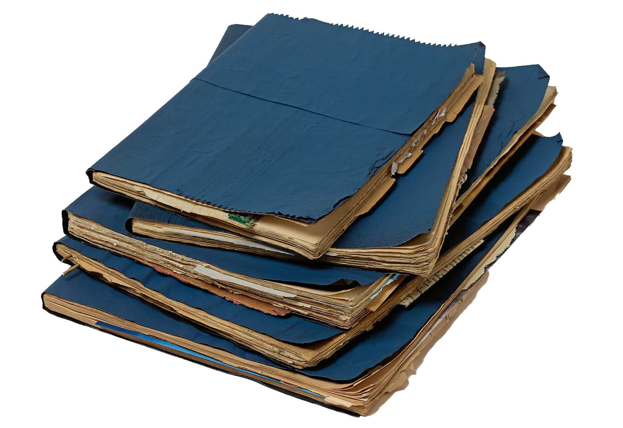
프란츠 카프카, 「여덟 권의 청색 팔절판 노트」 중 제1권

17 Jun 2025

「여덟 권의 청색 팔절판 노트_{Acht blaue Oktavhefte}」는 1917년 말부터 1919년 중순까지 카프카가 작성한 일련의 노트이다. 「팔절판 노트」라는 이름은 카프카의 출판 담당자인 막스 브로트가 그의 사절판 일기장과 구분하기 위해 붙인 것이다. 이후 브로트가 카프카의 일기를 출판했을 때 「팔절판 노트」는 생략되었는데, 카프카의 다른 일기보다 철학적이고 문학적이라는 점에서 성격을 달리한다는 이유에서였다. 이로 인해 「팔절판 노트」는 카프카 특유의 사색적이고 몽환적인 성격에도 불구하고 세간에 잘 알려져 있지 않으며, 특히 국내에서는 전문이 번역된 바가 없다. 이에 필자가 직접 번역을 시도했다. 비전공자의 번역인 점을 감안하여 독일어 원문을 같이 수록했다.

i.

모든 사람은 자신의 내면에 하나의 방을 가지고 다닌다. 이 사실은 심지어 청각의 감각을 통해 증명할 수 있다. 주위가 고요한 밤중에, 서둘러 걸음을 재촉하는 자가 귀를 기울일 때면, 그는 예컨대 벽에 충분히 고정되지 못한 거울이 부딪치는 소리를 듣는 것이다.

ii.

남자는 움츠린 가슴, 튀어나온 어깨, 축 늘어진 팔, 거의 들 수조차 없는 다리, 그리고 한 지점을 응시하는 눈빛으로 서 있다. 그는 화부_火夫다. 그는 삽에 석탄을 담아 화염이 치솟는 용광로에 던져 넣는다. 한 아이가 공장의 스무 안뜰을 살금살금 건너와 그의 거적때기에 안긴다. “아버지” — 아이가 말한다 — “제가 수프를 가지고 왔어요.”

iii.

이곳이 저 아래 겨울의 대지보다 따뜻한가? 백색은 온 주위에 쌓여가 오직 나의 들통만이 검다. 이전에 높은 곳에 있었던 나는 이제 깊은 곳에 있으며, 산을 올려다보려는 시도는 나의 목을 골절시킨다. 얼어붙은 백색은 사라진 스케이터들의 궤도를 따라 사방으로 금이 달렸다. 깊고 한 치도 꺼지지 않는 눈 위로, 나는 작은 북극견들의 발자국을 좇는다. 말을 타는 일은 의미를 잃었다. 나는 내려서 들통을 어깨에 메고 걷는다.

iv.

V. W.
베토벤 책에 대해 진심 어린 감사를 보냅니다. 쇼펜하우어는 오늘 시작합니다. 이 책들은 정말 대단한 업적입니다. 당신이 당신의 섬세한 손길과, 참된 진실을 향하는 강렬한 시선과, 절제되었으면서도 위엄한 대지의 불 같은 시적 본성과, 환상적일 정도로 방대한 지식을 통해 앞으로도 이러한 위업을 이룩하여 저에게 형언할 수 없는 기쁨을 주시기를 기원합니다.

v.

늙고 비대한 육신 속에서, 나는 가벼운 심장 질환을 앓으며, 점심 식사 이후 한 발은 바닥에 떨군 채 소파에 누워 역사책을 읽고 있었다. 하녀가 오더니 삐죽 튀어나온 입술 위로 두 손가락을 얹고는 방문객이 왔다고 일렀다.

“누구인가?” 나는 오후의 커피를 마셔야 할 때에 방문객을 상대해야 한다는 사실에 짜증이 난 목소리로 물었다. “중국인 남자입니다.” 하녀가 말하더니, 경련적으로 몸을 돌리고는 문 앞의 방문객이 들어서는 안 될 웃음을 삼켰다.

“중국인? 나를 보기 위해? 중국 의상을 입고 있나?” 하녀는 여전히 웃음을 억누르며 고개를 끄덕였다. “그에게 나의 이름을 말해주고, 그가 정말로 나를 방문하려는지 물어보거라. 나는 옆집 사람에게도 낯선 이인즉 중국에서는 오죽하겠나.”

하녀는 나에게 몸을 기울이더니 속삭였다. “그는 한 장의 쪽지만을 가지고 있는데, 쪽지에는 그를 들여보내달라는 부탁만 쓰여 있었습니다. 그는 독일어를 할 줄 모르며 알아들을 수 없는 언어로만 말합니다. 저는 쪽지를 그에게서 가져가는 것이 두려울 지경이었습니다.”

“그를 들여보내거라!” 나는 심장 문제가 종종 일으키곤 하는 숨가쁨 속에서 외치며, 책을 바닥 위로 던지고는 하녀의 어색한 접대를 저주했다. 나는 일어나 이처럼 천장이 낮은 방으로 들어오는 방문객이라면 누구든지 경악할 수밖에 없을 거구를 뻗으며 문에 다가섰다. 과연 그 중국인은 나와 눈이 마주치자마자 즉시 들어왔던 길로 미끄러지듯이 돌아갔다. 나는 사뿐히 복도로 손을 뻗어 남자의 비단 저고리를 움켜잡아 내게로 조심히 끌어당겼다. 그는 한눈에 보기에도 학자였으며, 작고, 연약했고, 뿔테 안경을 썼고, 얇고 희끗희끗하고 푸석한 염소 수염을 달고 있었다. 호감상의 난쟁이 — 머리는 한쪽으로 기울인 채 반쯤 감은 눈으로 미소 짓는구나.

vi.

어느 날 아침, 변호사 부케팔루스 박사는 그의 가정부에게 침대로 오게 하고는 그녀에게 말했다. “오늘 내 동생 부케팔루스 대 트롤해타 사_社 소송의 큰 재판이 있소. 나는 원고의 편에서 법정에 서지요. 재판이 적어도 수일은 걸릴 테다가, 정말이지 휴식 시간이 없을 것이니, 다음 며칠 동안 나는 집에 전혀 오지 않을 거요. 소송이 끝나거나, 끝날 조짐이 보이는 대로 전화를 주겠소. 지금으로서는 더이상 말할 수도 없고, 어떠한 질문에도 답할 수 없소. 당연히 내 목소리를 최대의 역량으로 보존하는 데 집중해야 하니 말이오. 그런 연유로, 나에게 아침 식사로 두 개의 날달걀과 꿀을 섞은 차를 가져다주겠소?” 그리고, 천천히 등을 베개 속에 묻히며, 눈 위를 손으로 덮은 채, 그는 침묵에 빠졌다.

수다스러울지언정 집주인 앞에 설 때면 두려워 죽을 지경이던 가정부는 이에 실로 당황했다. 그토록 놀라운 소식은 그리 갑작스럽게도 찾아오는 것이었다. 바로 전날 저녁만 하더라도 집주인은 그녀와 말 몇 마디를 나누었건만 곧 다가올 일에 관해서는 아무런 내색도 비치지 않았다. 하지만 재판 일정이 밤중에 정해졌을 수는 없지 않은가? 그리고 날밤을 새우면서 쉼 없이 진행되는 재판이 있던가? 그리고 왜 집주인은 이전에는 일절 알려준 적 없는 피고와 원고의 이름을 언급한 것인가? 그리고 작은 청과물 상점을 운영하는 집주인의 동생 아돌프 부케팔루스가 — 그나저나 그는 집주인과 지난 오랜 기간 좋은 관계로 보이지는 않았다 — 도대체 어떠한 거대한 소송에 연루되었다는 것인가? 그리고 집주인 앞으로 형언하기 힘들 정도의 시련이 닥쳤다는 사실이, 지금 그가 — 이른 새벽빛이 착시를 일으키는 것이 아니라면 — 초췌해진 자신의 얼굴을 손으로 가리는 모습과 어울린다고 정녕 말할 수 있는가? 그리고 그가 늘 원하던, 기력을 완전히 충전시켜 줄 약간의 와인과 햄은 막론하고 오직 차와 달걀만 받고자 한 것은? 그런 생각을 하며 가정부는 부엌으로 물러가, 그녀가 가장 좋아하는, 꽃과 카나리아가 있는 창가의 자리에 잠깐 앉아, 빗장으로 잠긴 창문 너머로 반쯤 벌거벗은 채 함께 뛰놀며 씨름하는 두 아이가 보이는 안뜰 너머를 바라보더니, 이내 일어나 한숨을 쉬고는, 차를 내고, 선반에서 달걀 두 개를 꺼내, 식사를 쟁반에 정돈하고, 차마 어쩔 수 없어 와인 한 병도 준비한 채, 모든 것을 침실로 가져갔다.

방은 비어 있었다. 어떻게, 집주인이 벌써 떠났을 리는 없을 텐데? 단 일 분 만에 옷을 입을 수는 없지 않은가? 하지만 그의 속옷과 양복은 어디에도 보이지 않았다. 도대체 집주인은 뭐 하자는 것인지 환장할 노릇이다. 서둘러 복도로! 코트, 모자, 그리고 지팡이조차 없다. 그렇다면 창문으로! 맙소사, 저기 대문을 나서는 집주인이 있다 — 머리 뒤로 모자를 걸치고, 코트 앞섶은 풀린 채, 손은 서류가방을 꽉 쥐었고, 주머니에 꿴 갈고리 위로 지팡이는 대롱거린다.

vii.

당신은 파리의 트로카데로를 아십니까? 사진만 봐서는 전혀 짐작하지 못할 크기를 자랑하는 이 건물에서, 아주 대단한 재판의 핵심 심리가 지금 이 순간 진행되고 있습니다. 어쩌면 당신은 그토록 큰 건물을 어떻게 이처럼 지독한 겨울에 난방하는 것이 가능한지 궁금할지도 모르겠습니다. 건물은 난방되지 않습니다. 이와 같은 경우에 난방부터 생각하기란, 당신이 인생을 보낸 곳과 같은 안락한 소도시에 사는 사람들에게나 가능한 일이죠. 트로카데로는 난방이 없지만 이것이 심리의 진행을 방해하지는 않습니다. 오히려 모든 방향에서 뿜어져 나오는 한기 속에서, 심리는 그에 정확히 부응하는 빠르기로 진행됩니다. 가로와 세로를 종횡무진 가르며.

viii.

어제 실신_失神이 나를 찾아왔다. 그녀는 이웃집에 산다. 나는 예전부터 저녁 무렵이면 종종 그녀가 몸을 굽히며 대문을 지나 사라지는 것을 보았다. 길게 흘러내리는 옷과 깃털이 꽂힌 넓은 모자를 쓴 거구의 여인. 그녀는 마치 죽어가는 환자에게 너무 늦게 도착한 것은 아닌지 두려워하는 의사처럼 급히 문을 열고는 소란스레 들어왔다. “안톤” — 그녀는 공허하면서도 자부하는 듯한 목소리로 외쳤다 — “제가 왔어요, 제가 여기 있어요!” 내가 가리킨 소파에 그녀는 기꺼이 털썩 주저앉았다.

“높이도 사는군요, 높이도 살아요.” 그녀는 신음하듯이 말했다.

나는 내 안락의자에 파묻힌 채 고개를 끄덕였다. 눈앞으로는 내 방으로 이어지는 수많은 계단이 끝없이 일렁이는 물결처럼 앞다투어 튀어 올랐다.

“어찌 이리도 춥나요?” 그녀는 묻더니, 헌 펜싱 장갑처럼 생긴 그녀의 기다란 장갑을 벗어 탁자 위로 던지고는 갸우뚱한 고개로 나를 바라보며 눈을 찡긋했다. 나로서는 한 마리의 참새가 된 듯한 기분이었으니, 계단 위에서 폴짝이며 날갯짓을 연습하는데 그녀가 나의 부드럽고 솜털 같은 회색 깃털을 헝클어뜨리는 것이었다.

“당신이 저에 대한 그리움으로 괴로워한다니 진심으로 유감이에요.” 그녀가 말했다. “이따금 당신이 안뜰에 서서 제 창문을 올려다볼 때면 당신의 피폐한 얼굴에서 깊은 슬픔을 읽곤 했지요. 그래요, 제가 당신에게 적의를 품은 것은 아니랍니다. 비록 당신이 제 마음을 아직 얻지 못했어도, 그것을 쟁취하는 것 또한 불가능하진 않으니까요.”

ix.

사람은 이토록 무관심에 빠질 수 있는가 — 그가 영원히 올바른 길을 잃어버렸다는 그토록 깊은 신념에.

x.

착오. 내가 연 것은 긴 복도 끝 위쪽에 있는 내 방의 문이 아니었다. “착오였습니다,” 라는 말과 함께 나는 다시 나가려고 했다. 그 순간, 나는 방 안쪽으로 수척하고 수염이 없는 사내를 보았다. 입을 굳게 다문 채, 그가 앉은 작은 탁자에는 단 하나의 석유 램프만이 있었다.

xi.

우리의 집 — 변두리에 위치한 이 거대한 건물, 지울 수 없는 중세의 폐허가 스며든 다세대 주택에서, 얼음 같은 안개가 낀 금일의 겨울 아침 이런 공문이 게시되었다.

모든 세입자께 알립니다.

나는 다섯 자루의 장난감 총을 가지고 있습니다. 총은 저마다 고리에 걸린 채 내 장롱에 보관되어 있습니다. 첫 번째 총은 나의 것이지만 나머지는 원하는 사람이 가져가도 좋습니다. 네 명보다 많은 희망자가 있을 시 자신이 소유한 총을 가져 와 장롱에 두어야 합니다. 통일성은 반드시 지켜져야만 하기 때문입니다. 통일성 없이는 우리는 앞으로 나아갈 수 없습니다. 그나저나 내가 가지고 있는 총들이란 죄다 어떤 용도로도 쓸모가 없습니다. 기계 장치는 망가졌고, 노리쇠는 떨어져 나갔으며, 오직 방아쇠만이 여전히 딸깍거릴 뿐입니다. 그러니 필요하다면, 이런 총을 더 많이 구하기란 어려운 일이 아닐 것입니다. 하지만 근본적으로 보면, 첫 시도에는 총이 없는 사람들도 괜찮을 듯합니다. 우리 총을 가진 사람들이 결정적인 순간에 무장하지 않은 자들을 가운데로 몰아넣을 것입니다. 이 전투 방식은 최초의 미국 농부들이 인디언들과 맞설 때 증명된 방법인 만큼, 상황의 유사성을 고려할 때 여기서도 통하지 않을 리 있겠습니까? 생각해 보면 우리는 심지어 오래도록 총을 포기할 수도 있고, 이 다섯 자루조차 꼭 필요한 것은 아닙니다만, 단지 이미 존재하기 때문에 쓰자는 것뿐입니다. 하지만 다른 네 사람이 총을 들기를 원하지 않는다면, 그렇게 하지 않아도 됩니다. 그러면 나 혼자서만 지도자로서 총을 들겠습니다. 그러나 우리는 지도자를 가져서는 안 됩니다. 그래서 나 또한 내 총을 부수거나 내려놓을 것입니다.

이것이 첫 번째 공문이었다. 우리의 집에 사는 사람들은 시간도 없고 공문을 읽거나 숙고할 의욕도 없다. 얼마 안 있어 그 종이쪼가리는 다락방에서 시작해 복도로 터져 나온 더러운 물줄기에 흠뻑 젖은 채로 계단을 따라 쓸려 나가더니 그곳 밑에서 역류하는 물줄기와 싸우는 신세가 되었다. 그러나 일주일 뒤 두 번째 공문이 붙었다.

세입자들이여!

지금까지 아무도 나에게 연락하지 않았습니다. 나는 내 생계에 필수적인 일을 하지 않는 시간에는 항상 집에 머물러 있었습니다. 집을 비울 때는 방문을 열어두어, 원하는 사람은 누구든 이름을 적을 수 있도록 책상 위에 종이를 놓아두었습니다. 아무도 이름을 적지 않았습니다.

xii.

가끔씩 나는, 내가 기계공장에서의 교대근무를 마치고 밤늦게 또는 이른 아침에 집으로 돌아올 때, 내가 저지른, 그리고 저지를, 과거와 미래의 모든 죄가 뼈마디의 통증으로 속죄되는 것은 아닌지 생각한다. 나는 내가 이 일을 견딜 수 있을 정도로 강하지 않다는 사실을 이미 오래전부터 알고 있다. 그러나 나는 아무것도 바꾸지 않는다.

xiii.

우리의 집 — 변두리에 위치한 이 거대한 건물, 중세의 폐허가 스며든 다세대 주택에는, 나와 같은 복도에서 한 노동자 가족과 같이 사는 서기가 있다. 사람들은 그를 공무원이라고 부르지만 실상은 하찮은 서기에 불과하며, 낯선 부부와 그들의 여섯 자식 틈에 끼인 채 바닥에 깔린 밀짚 둥지에서 밤을 보내는 자이다. 그리고 그가 그토록 하찮은 서기라면, 내가 그에게 무슨 신경을 쓰겠는가. 이 집 — 도시가 끓여낸 불행이란 불행은 다 모인 이 집에도, 적어도 백 명은 넘는 사람들이 살거늘…

xiv.

나와 같은 복도에는 한 수선재봉사가 산다. 아무리 조심해도 내 옷은 너무 빨리 닳아서, 최근에도 나는 그에게 다시 외투 하나를 들고 가야만 했다. 그날은 참으로 아름답고 따뜻한 여름 저녁이었다. 재봉사는 자신과 아내, 그리고 여섯 아이까지 모두 단 한 칸의 방 — 그 방은 부엌이기도 하다 — 에서 살고 있다. 그런데도 그는 심지어 한 세무청의 서기를 세입자로 들였다. 이 정도로 들어찬 방은 이미 열악하기 짝이 없는 우리 주택의 기준으로 봐도 지나친 수준이다. 그렇다고는 해도 사람은 각자의 사정이 있고, 재봉사에게 또한 그의 절약에 달아날 수 없는 이유가 분명히 있겠거니, 외부인이 그 이유에 대해 굳이 이야기하려는 일은 없다.

xv.

1917년 2월 19일.

오늘은 헤르만과 도로테아, 그리고 리히터 회고록 약간을 읽었으며, 그의 사진들을 봤고, 마지막으로 하웁트만의 그리젤다에서 나오는 장면을 읽었다. 한 시간이라는 순간 안에 나는 다른 사람이 되어 있었다. 모든 풍경은 여전히 안개처럼 뿌옇지만, 이제는 안개 그림으로 변했다. 오늘 처음 신어 보는 질긴 장화 속에는 — 그 장화는 원래 군사용으로 만들어진 것이었다 — 또다른 사람이 서 있었다.

xvi.

저는 크룸홀츠 씨 댁에 삽니다. 방은 세무청의 한 서기와 나눠 쓰지요. 그 방에서는 크룸홀츠 씨의 두 딸 — 여섯 살, 일곱 살 소녀입니다 — 또한 같은 침대에서 잡니다. 서기가 이사를 해온 첫날부터 — 저로 말하자면 이미 수년 동안 크룸홀츠 씨 댁에 살고 있었습니다 — 저는 그의 첫인상에서 석연찮은 수상함을 느꼈습니다. 평균 신장 이하의 남성. 허약한 체격과, 건강하다고는 할 수 없는 폐. 후줄근한 회색 옷가지. 나이를 가늠할 수 없는 주름진 얼굴. 귀를 덮도록 넘겨진 회갈색의 긴 머리카락. 코끝까지 내려온 안경. 그리고 작고 — 역시나 — 회색인 염소 수염.

xvii.

내가 중부 콩고에서 철도 공사에 종사하며 보냈던 삶은 즐거운 것이 아니었다.

나는 내 오두막집의 차창이 쳐진 베란다에 앉아 있었다. 한쪽으로는 긴 벽 대신 극도로 촘촘한 모기장이 쳐져 있었는데, 그것은 현장 감독관 중 한 명이자 우리의 철도가 지나가는 지역의 족장에게서 얻은 것이었다. 삼베로 만든 그 그물은 튼튼하면서도 섬세하여, 유럽에서는 결코 만들 수 없을 정도였다. 그것은 내 자랑거리였고 많은 이들의 부러움을 샀다. 그 그물이 없었더라면 이렇게 저녁에 베란다에 평화롭게 앉아, 지금처럼 불을 켜고, 오래된 유럽 신문을 샅샅이 펼쳐 읽으며, 파이프를 힘차게 피우는 일은 결코 불가능했을 것이다.

xviii.

나는 — 누가 자신의 능력을 이토록 자부하며 말할 수 있겠는가 — 행복하며 지칠 줄 모르는 늙은 낚시꾼의 손목을 가지고 있다.

나는 예컨대 집에 앉아, 낚시하러 나가기 전에, 고개를 휙 돌려 오른손을 응시하고는, 한 번은 멀리, 한 번은 가까이 손을 거둔다. 그것만으로도 나는 다가올 낚시의 결과를, 때로는 세세한 부분까지도, 내 시각과 촉각 속에서 예지할 수 있다. 평상시에는 힘을 비축하도록 금팔찌 속에 가둬 두는 이 날렵한 손목의 육감. 나는 내 낚시터의 강물을 구체적인 시각의, 구체적인 물살 속에서 본다. 강의 단면이 내 앞으로 드러난다. 분명한 수와 종류로 열 군데, 스무 군데 — 백 군데 지점에서 물고기들이 단면을 향해 밀려오는 모습이 보인다. 이제 나는 어떻게 낚아야 할지를 안다. 어떤 녀석들은 머리로 그 단면을 파고들어 가거늘, 나는 그들 앞에서 낚싯대를 흔들어댈 뿐인데 그들은 낚시고리에 걸려버린다. 내가 집의 책상에 앉아 있을 때도 황홀감을 안겨주는 운명의 순간. 다른 물고기들은 배_腹까지 단면에 닿으니 그때가 절정의 기회이다. 나는 몇몇은 여전히 낚아내지만, 다른 물고기들은 꼬리까지 미끄러뜨리며 위험천만한 단면을 지나 내게서 빠져나가고 만다. 하지만 오직 이번뿐이다 — 진정한 낚시꾼은 어떤 물고기도 놓치지 않거늘.

---

서두의 이미지는 막스 리히터, The Blue Notebooks 의 앨범 커버이다.

Franz Kafka, The Blue Octavo Notebooks, Volume 1

17 Jun 2025

This post is originally a Korean translation of Kafka’s The Blue Octavo Notebooks. Given that there already exists an English translation of the work, I won’t go through the hassle of translating into English again. However, I present the following passage, which I particularly admire.

이탈리안 게임

12 Jun 2025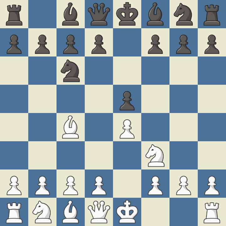

1. e4 e5
2. Nf3 Nc6
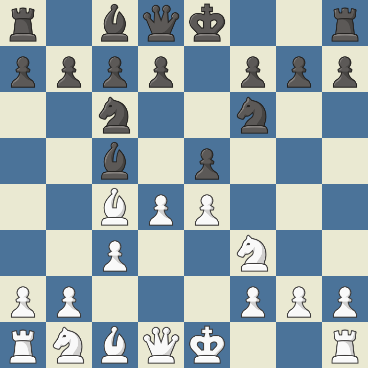
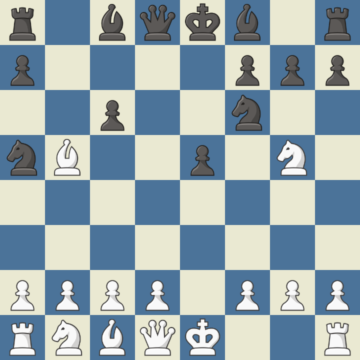
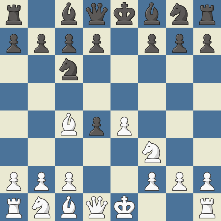
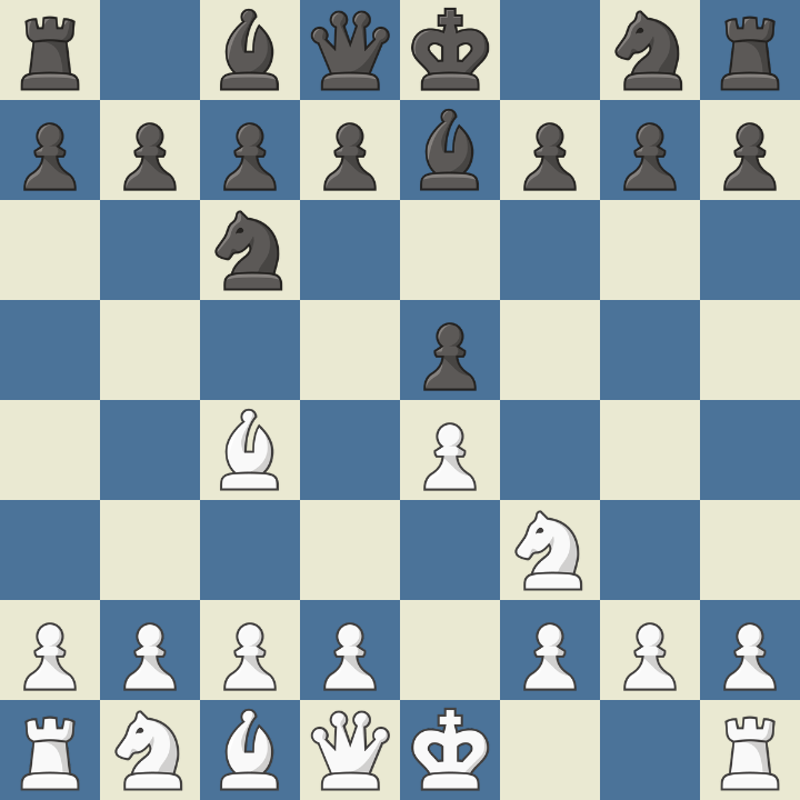
3. Bc4

해당 오프닝을 이탈리안 게임이라고 한다. 백의 아이디어는 흑의 d5를 저지함으로써 강하게 중앙을 컨트롤하는 것이다. 이에 대해 흑은 소극적으로 대응해서는 안 된다. 예를 들어 …h6 (안티 프라이드 리버 어택: 백의 Ng5, Bg5를 저지하는 수)은 권장되지 않는다. 백이 4. d4를 쳤을 때 백의 중앙이 너무 강해지기 때문이다. 흑이 4. ..exd4로 대응할 경우 백은 5. Nxd4로 되잡는다.

만약 흑이 5. …Nxd4로 나이트까지 교환한다면 백의 6. Qxd4가 강력하다. 흑은 퀸사이드 나이트를 교환했기 때문에 백의 퀸을 쫓아낼 마땅한 방법이 없을 뿐더러 백의 비숍과 퀸에 의해 킹사이드가 노려지고 있어 전개가 상당히 까다로워진다.

3. Bc4에 대한 흑의 정석적인 대응은 두 가지이다.

3. …Bc5

백의 d4를 저지하는 수이다. 이제 백은 d4를 치기 위해 추가적인 지지가 필요하기 때문에 4. c3로 d4를 준비한다. 이 라인을 지우코 피아노라고 부른다. 흑의 정석적인 대응은 …Nf6이다. 백에게 d4를 칠 기회를 주지만, 대신 흑은 e4를 노릴 수 있다. 백은 두 가지 선택지가 있다.

수비적 플레이: 5. d3

백은 e4의 위협을 d3로 수비한다. 이 라인을 지우코 피아니시모이라고 부른다. 이후 백은 킹사이드 캐슬링을 진행하고 나머지 마이너 피스를 전개하여 게임을 안정적으로 운영한다.

공격적 플레이: 5. d4

백은 e4의 위협에 개의치 않고 d4를 친다. 이 라인을 지우코 피아노 메인이라고 부른다. 메인 라인을 들어가게 되면 기물들이 중앙에서 치열하게 뒤엉켜 싸우는 복잡한 게임이 펼쳐진다.

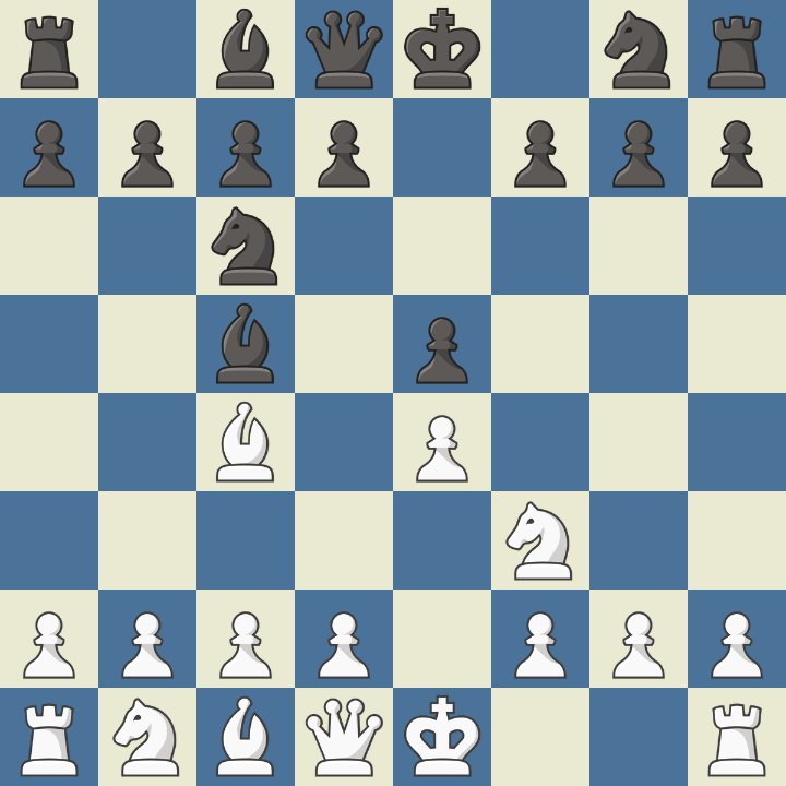
3. …Nf6

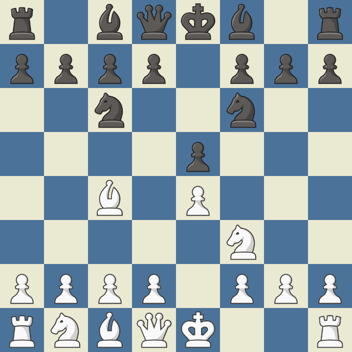
백의 e폰을 공격하는 동시에 d5를 지지함으로써 d5 폰브레이크를 준비하는 수이다. 이 라인을 투 나이트 디펜스라고 부른다. 여기서도 백은 선택지가 있다.

수비적 플레이: 4. d3

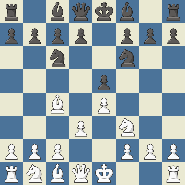
e폰을 수비하는 동시에 어두운 비숍의 길을 열어주는 수이다. 이후 백은 지우코 피아니시모와 마찬가지로 킹사이드 캐슬링을 진행하고 나머지 마이너 피스를 전개한다.

공격적 플레이: 4. Ng5

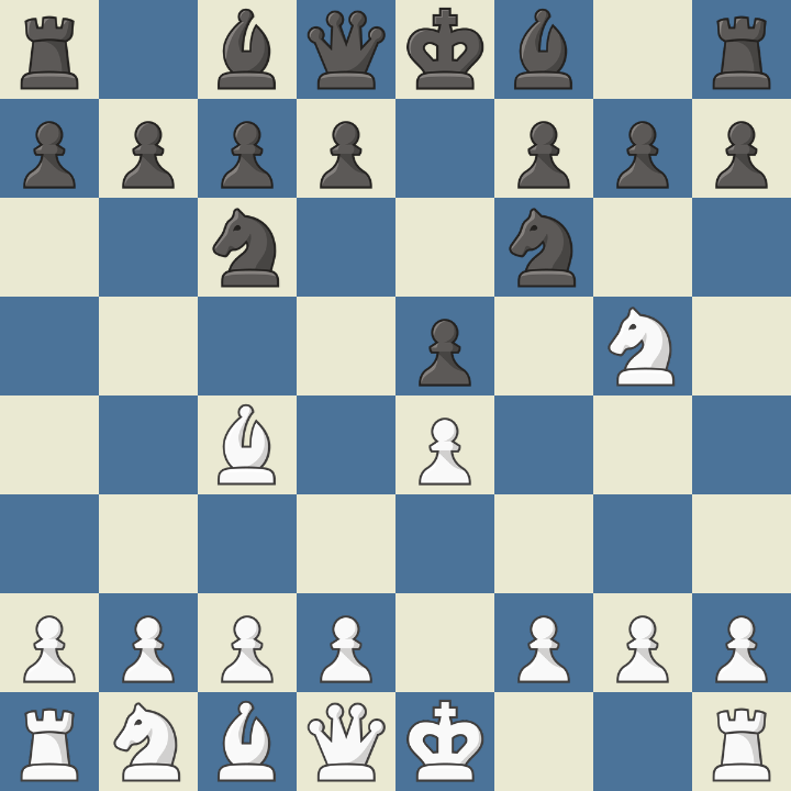
Nf7로 퀸과 룩을 포크하는 공격을 준비하는 수이다. 이것을 이탈리안 게임 나이트 어택 바리에이션이라고 한다. 흑의 유일하게 올바른 대응은 d5이다. Bc5 (트렉슬러 카운터어택) 등으로 흑이 역공을 노리는 라인이 있지만, 이 경우 백이 나이트로 공격하는 대신 Bf7+로 킹사이드를 무너뜨리고, Bb3로 안전하게 후퇴하면 된다.

…d5에 대해 백이 5. Bb3 등으로 비숍을 빼면 전개가 너무 느리기 때문에, 5. exd5가 바람직하다. 반면 5. Bxd5는 블런더이다. 5. …Nxd5 6. exd5로 나이트와 비숍이 교환되면 …Qxf5로 나이트가 잡힌다. 백 또한 7. dxc6로 나이트를 잡을 수 있기는 하지만, 이 경우 …Qxg2로 퀸이 킹사이드 진영에 침투하는 것을 막을 수 없다.

5. exd5에 대한 흑의 대응은 흔히 두 가지이다.

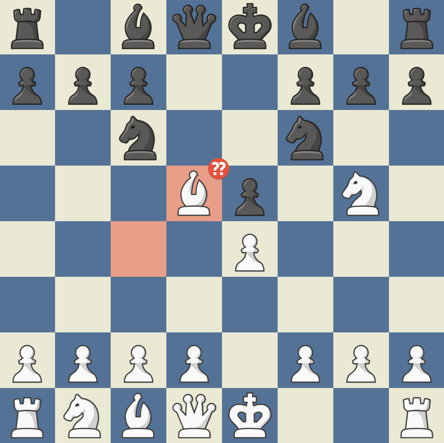
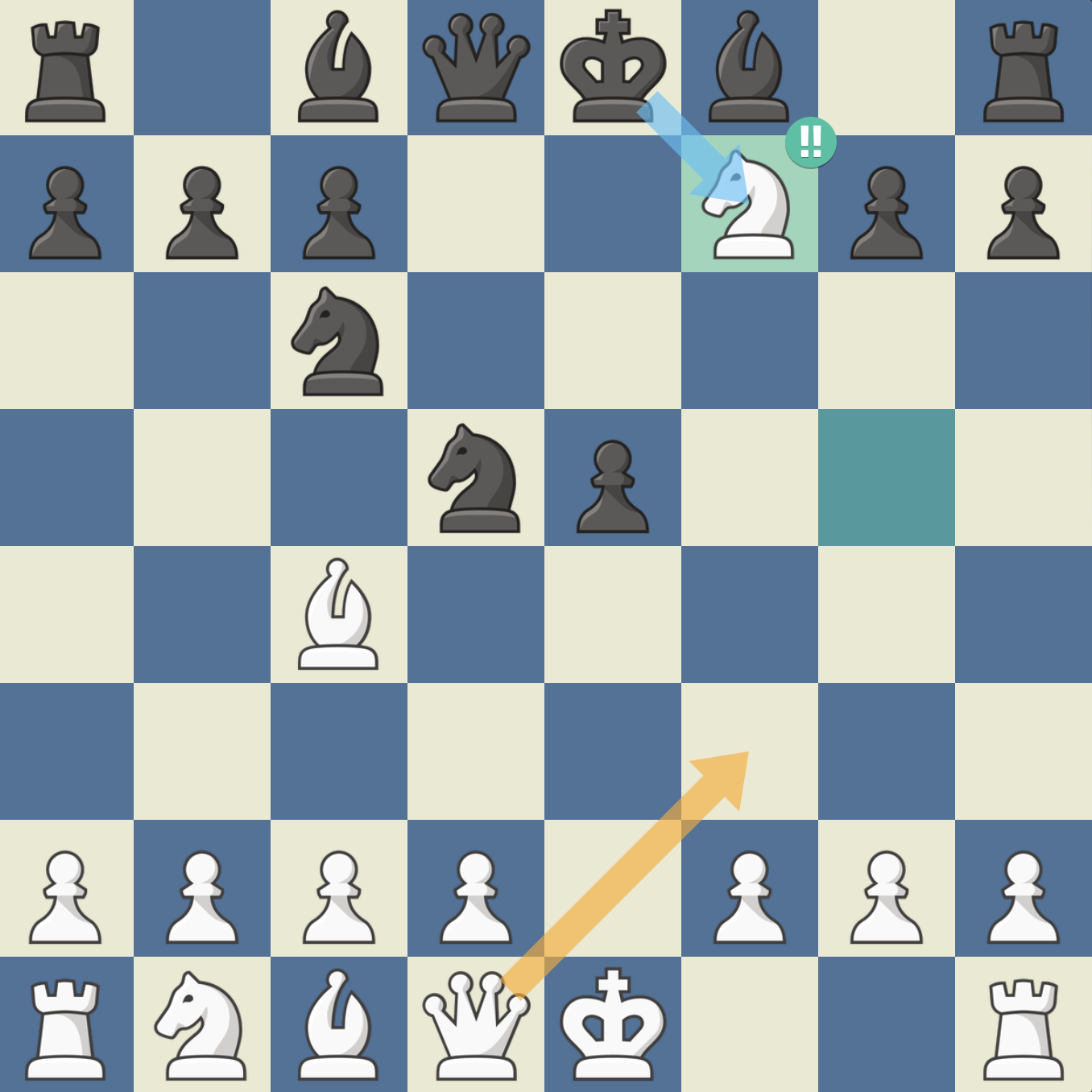
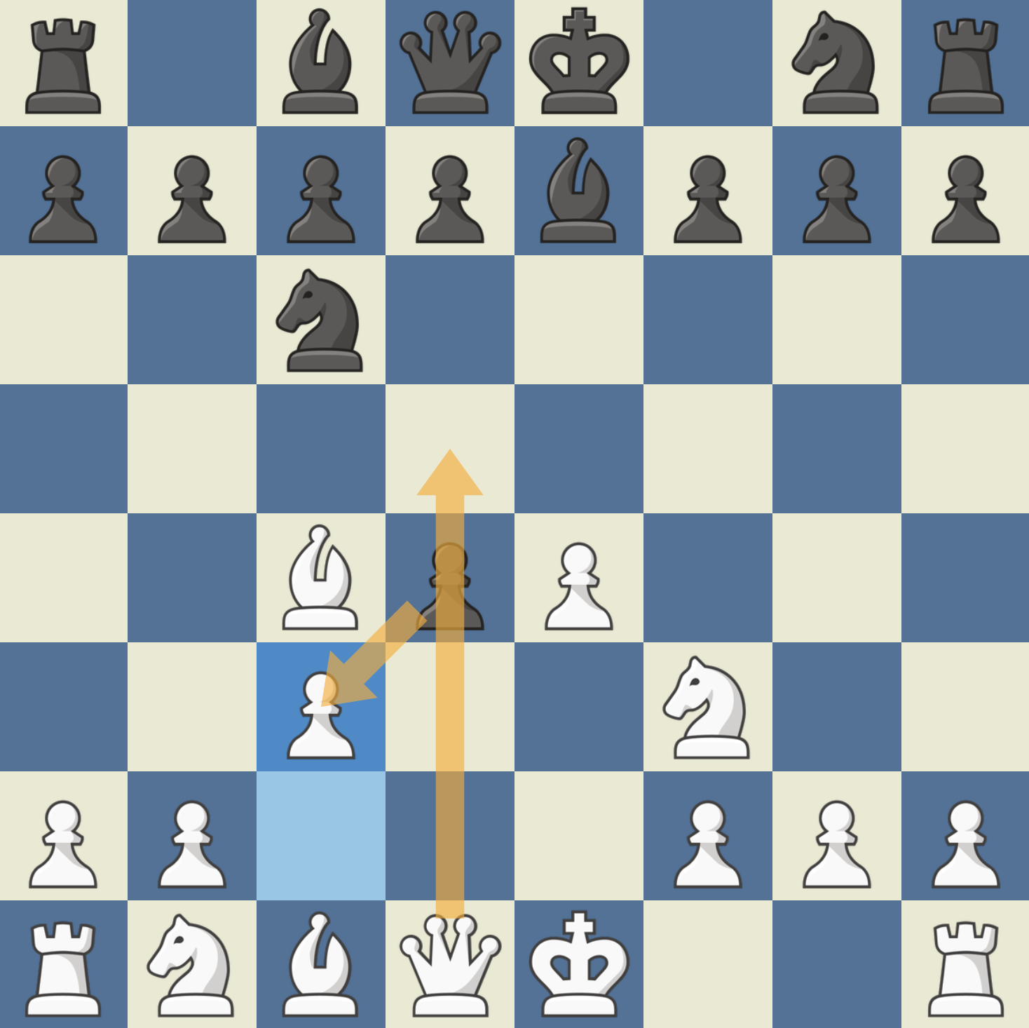
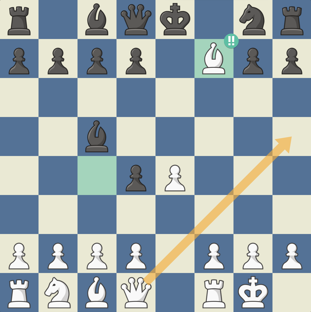
5. …Nxd5

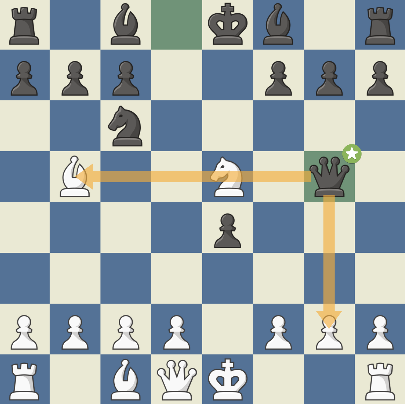
흑의 의도는 나이트에 대한 퀸의 공격을 드러내면서 폰을 회수하는 것이다. 그러나 이것은 초보자 경기에서 정말 많이 나오는 실수이다. 백의 강력한 수, 6. Nxf7!!이 있다. 이것을 프라이드 리버 어택이라고 부른다. 흑이 …Kxf7으로 나이트를 잡으면 백은 7. Qf3+로 체크와 동시에 d5 나이트를 공격한다. 여기서 만약 흑이 Kg8으로 피하면 8. Bxd5가 2수 메이트이다.

5. …Na5

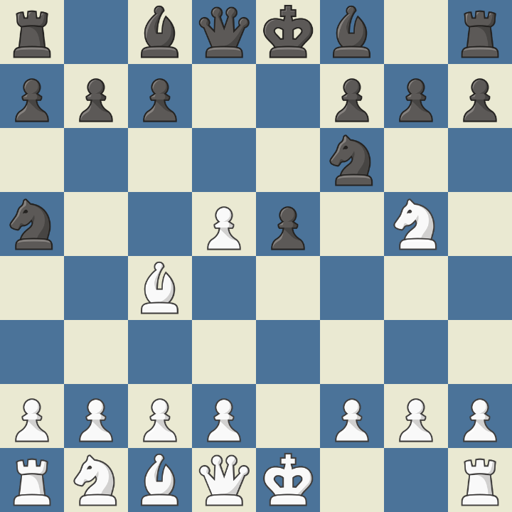
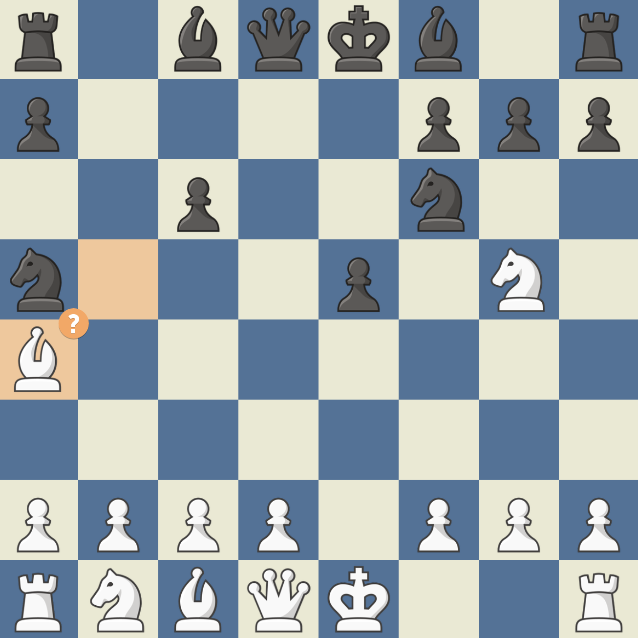
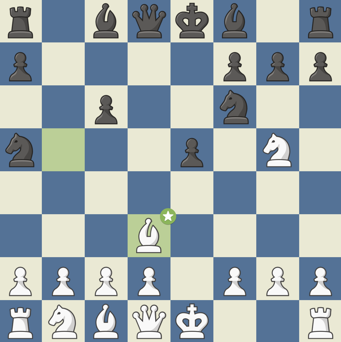
나이트가 비숍을 공격하는 폴레리오 디펜스이다. 백의 정석적인 대응은 6. Bb5+로 …c6를 유도하고, 7. dxc6 bxc6로 폰을 교환하는 것이다. (흑이 7. …Nxc6로 되잡을 경우 백은 8. Bc4로 돌아가서 다시 Nf7 공격을 노릴 수 있다. 물론 프라이드 리버 어택도 여전히 가능하다.) 결과적으로 흑은 비숍길이 열리고 중앙에 폰이 있다는 포지션적 이점을 가지는 반면, 백은 원폰업이라는 이점을 가지게 된다.

7. …bxc6로 비숍이 공격받았으므로 백은 비숍을 빼야 하는데, Ba4로 뺴는 것은 블런더이다. (팁: 이거 두면 ‘바보_BaFour‘라고 외우면 된다) 흑의 8. …h6 나이트 공격이 강력하기 때문이다.

다음 경우의 수에서 보이듯이 백은 결국 킹사이드 진영이 망가지거나, 비숍-나이트 포크에 걸리거나, 나이트가 트랩 당하거나, 나이트를 원래 자리로 후퇴시키게 된다.

• 9. Nh3 Bg4 10. f3 Bxh3 11. gxh3 (킹사이드 붕괴)
• 9. Nf3 e4 (나이트 공격)
  • 10. Ne5 Qd4 (비숍-나이트 포크) 11. Bxc6+ Nxc6 12. Nxc6 Qd5 (나이트 트랩)
  • 10. Nh4 d5 (나이트 트랩)
  • 10. Ng1 (나이트 후퇴)

대신 백은 8. Be2, 8. Bd3 (9. Ne4), 8. Qf3 (9. Qxa8) 등으로 응수할 수 있다.

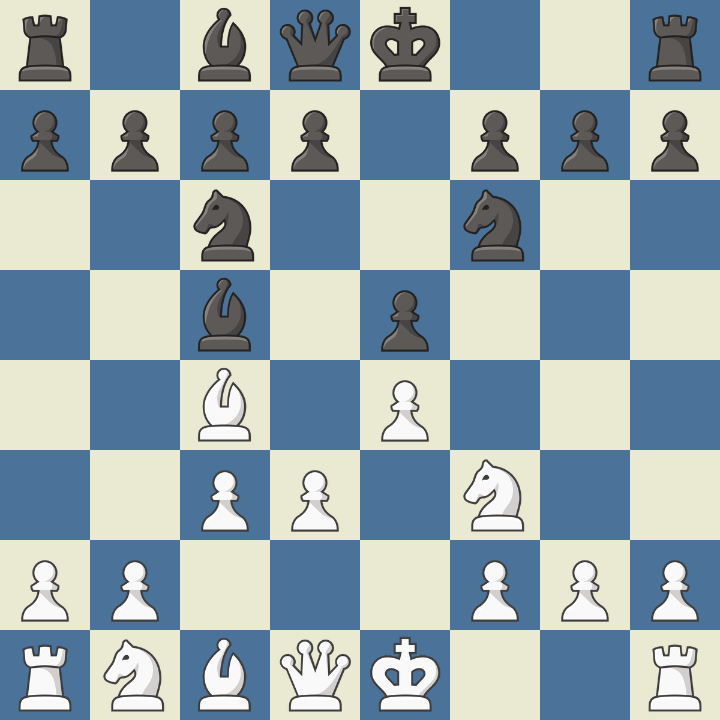
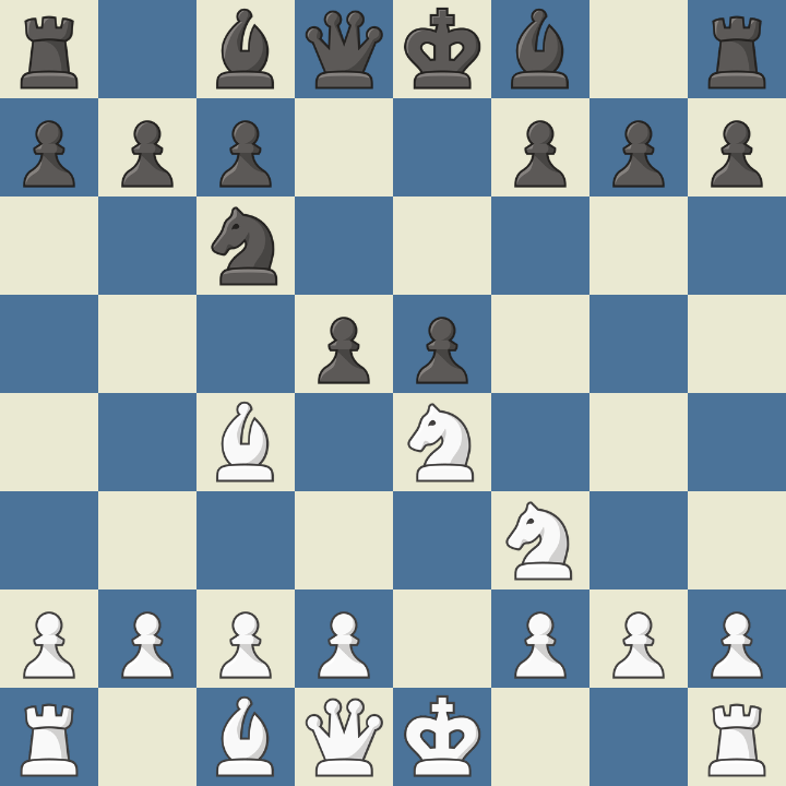
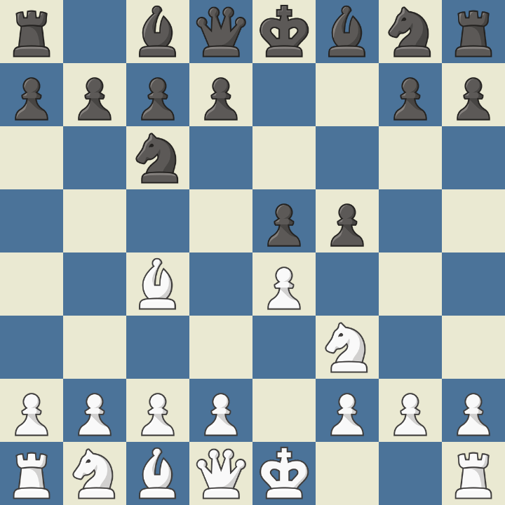
스카치 전환: 4. d4

Nxe4의 위협을 d4 폰브레이크로 맞받아치는 수이다. 흑이 4. …exd4로 대응할 경우 이는 스카치 갬빗에서 흑이 4. …Nf6로 대응한 것과 형태가 같다.

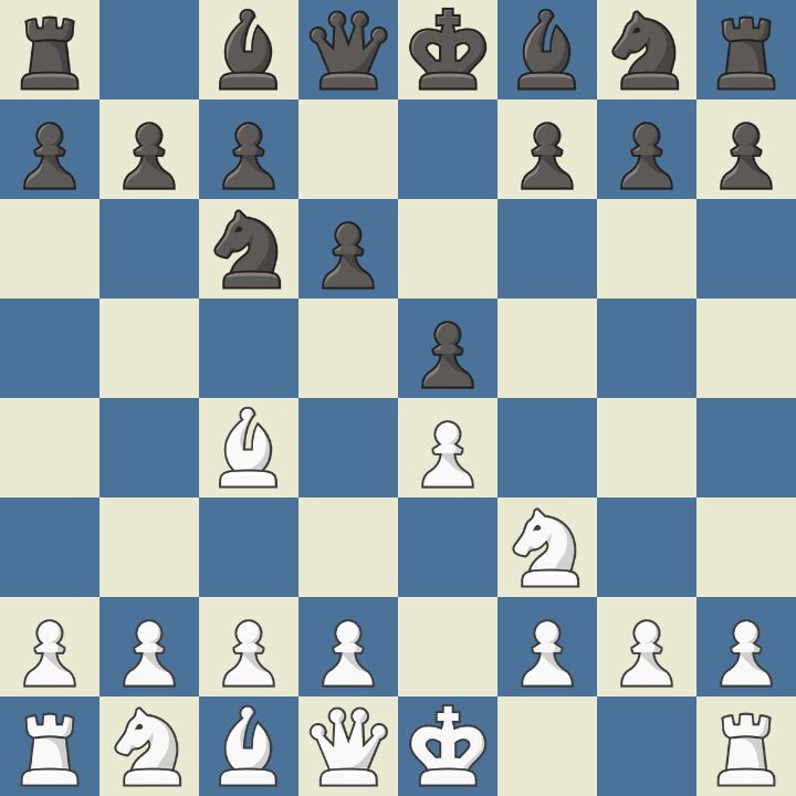
스카치 갬빗. 1. e4 e5 2. Nf3 Nc6 3. d4 exd4 4. Bc4

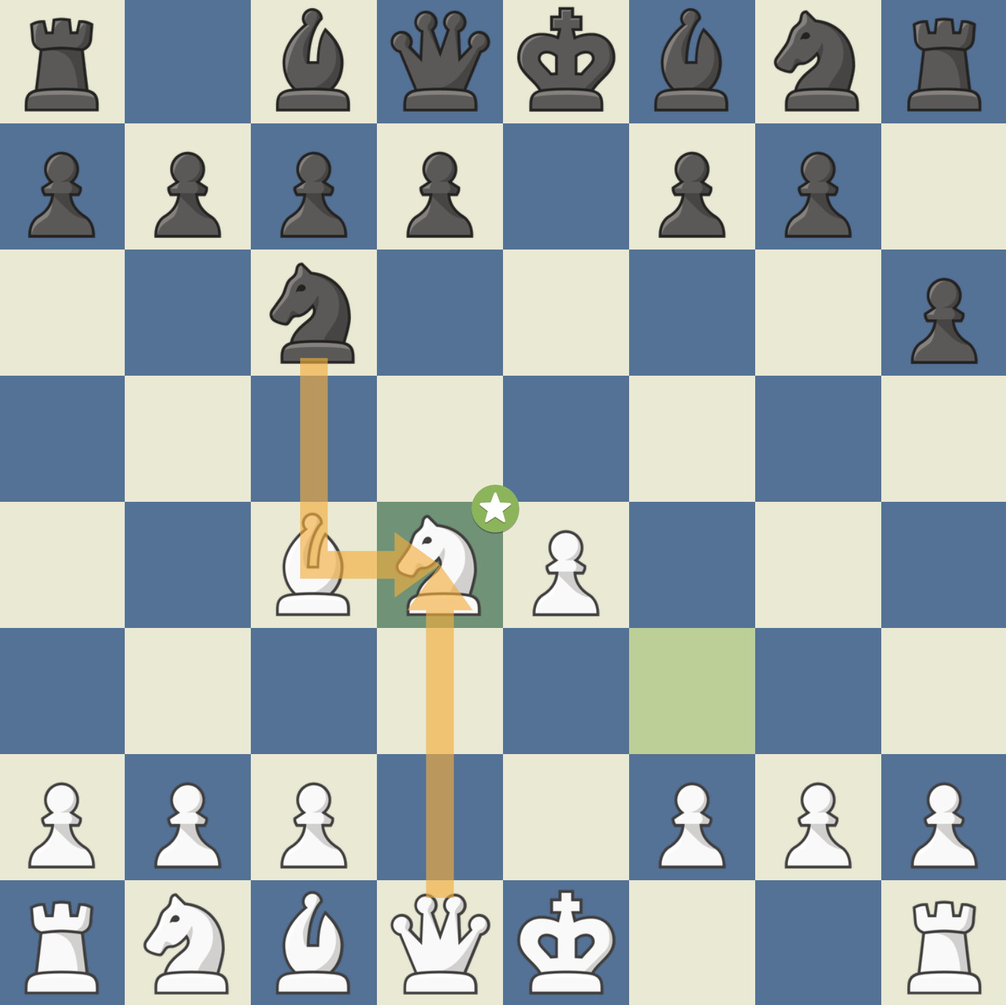
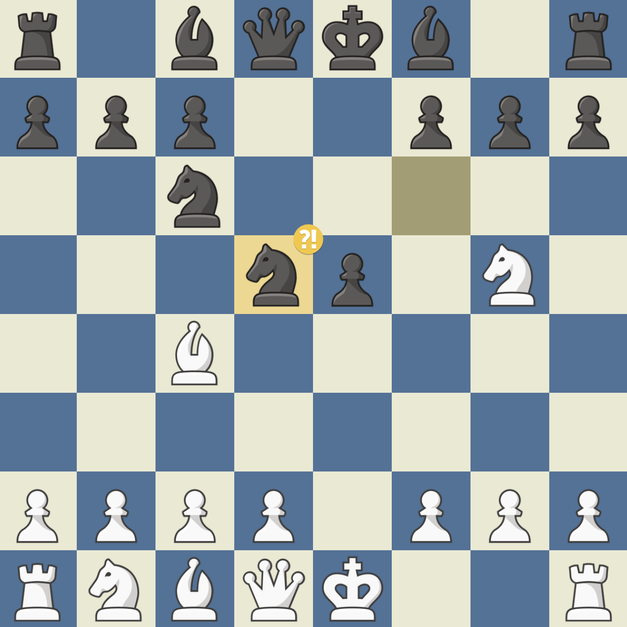
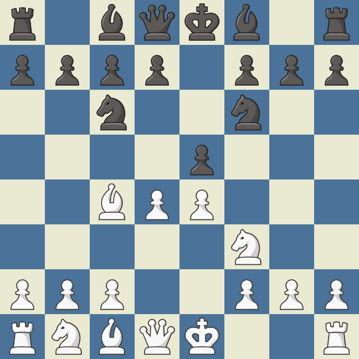
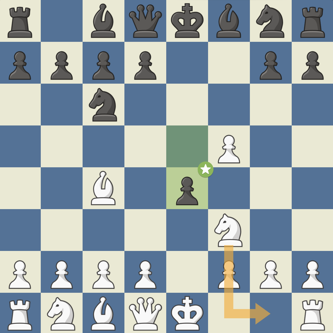
포 나이트 이탈리안: 4. Nc3

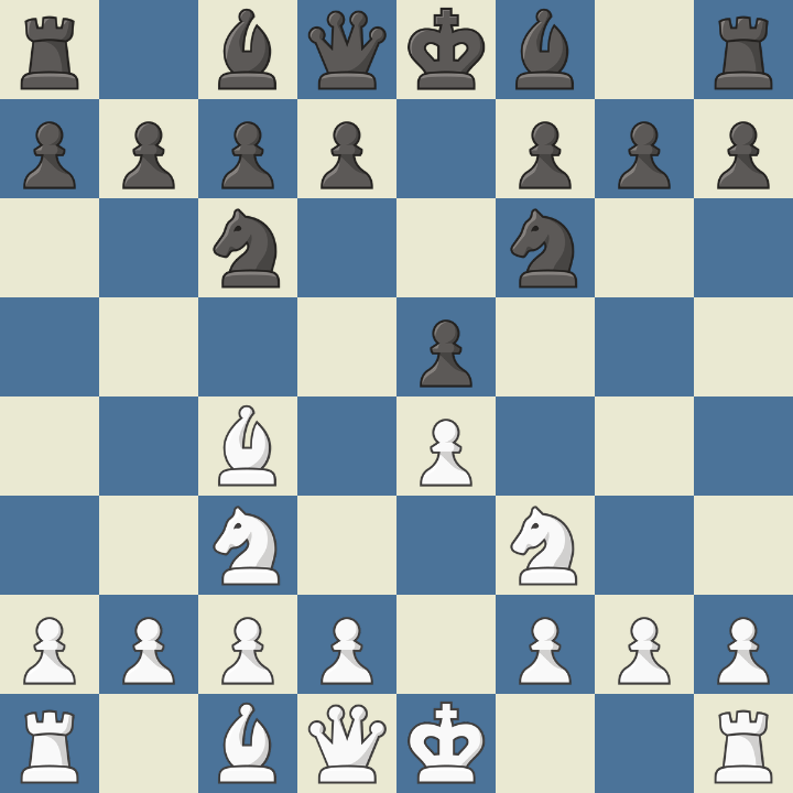
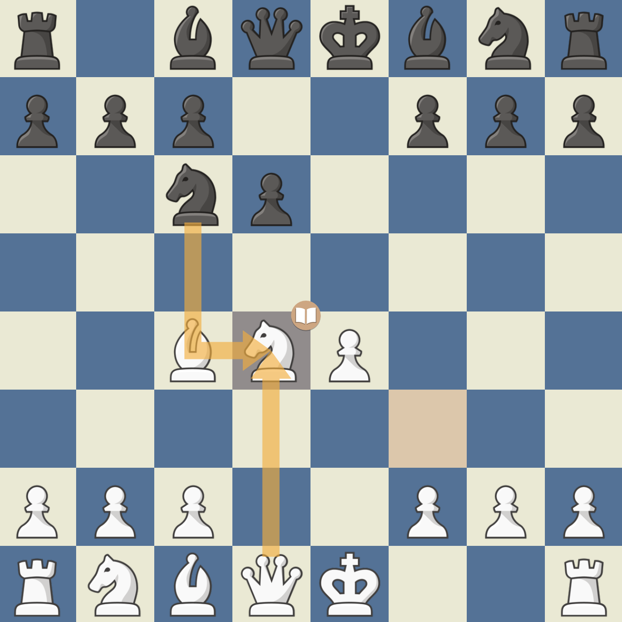
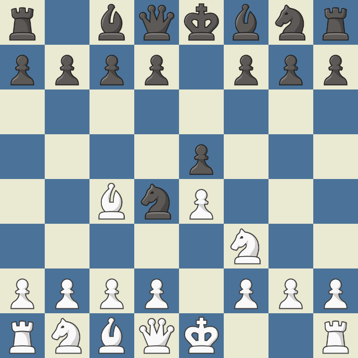
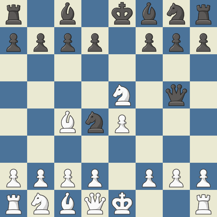
이 또한 초보자 경기에서 정말 많이 나오는 실수이다. 이 수의 아이디어는 나이트를 전개하는 동시에 e폰을 지키려는 것이나, 여기서 흑은 4. …Nxe4로 나이트를 희생할 수 있다. 백이 5. Nxe4로 나이트를 되잡으면 흑은 …d5를 쳐서 비숍과 나이트를 포크한다.

백이 대응하는 경우의 수를 살펴보자.

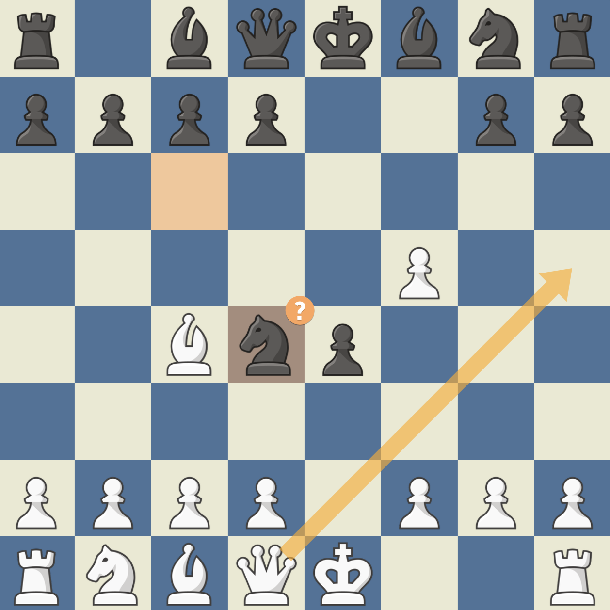
6. Bxd5

백이 데스페라도 전략으로 폰을 먹으면 흑은 …Qxd5로 회수한다. 이 경우 흑과 백은 기물 점수로는 동등하지만 백은 중앙 폰과 쌍비숍 이점을 잃었고, 흑의 퀸 전개까지 도와준 셈이기 때문에 포지션적으로 불리하다. (엔진 기준 -1.1점)

6. Bb5

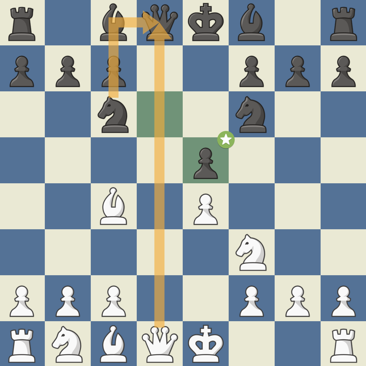
백은 나이트를 내주는 대신에 흑의 나이트를 핀에 건다. 나이트가 핀에 걸렸으므로 6. …dxe4 이후로 7. Nxe5가 가능할 것 같지만, 이 경우 백은 완전히 불리해진다. 흑이 7. …Qg5로 5 랭크의 나이트와 g폰을 동시에 공격할 수 있기 때문이다.

여기서 백이 당황해서 8. Bxc6를 두면 흑은 사실상 이기게 된다. 비숍이 킹 앞의 e2 칸을 더이상 보호하고 있지 않아, 다음의 치명적인 공격이 가능해진다.

1. …bxc6 9. Nxc6 Qxg2 10. Rf1 Bg4 11. f3 Bxf3 12. Rxf3 exf3

여기서 흑은 Qg1# 한수 메이트가 있기 때문에 백은 체크메이트를 피해야 한다. 그러나 체크메이트를 피한다 하더라도, f폰의 프로모션과 그로 인한 디스커버드 체크를 피할 수 없어서 사실상 흑이 이긴 게임이다.

---

이제 조금 더 드물게 나오는 라인을 알아보자.

3. …d6

e4 폰을 지키는 수이다. 이것은 필리도어 디펜스 (1. e4 e5 2. Nf3 d6) 이후 백이 비숍을 전개하고 흑이 나이트를 전개한 것과 형태가 같다.

이탈리안 필리도어 디펜스와 일반 필리도어 디펜스 모두 백의 대응은 d4를 치는 것이다. 이후 전개는 대략 다음과 같다.

흑이 exd4를 할 경우

백은 Nxd4로 되잡는데. 백은 센터 폰이 있고 나이트의 활동성이 좋다는 이점을 가진다. 반면 흑은 견고한 방어를 구축하게 된다.

흑이 exd4를 하지 않을 경우

이탈리안의 경우 Nc6 전개가 되어 있기 때문에 5. dxe4 dxe4 이후 6. Qxd8이 들어오더라도 …Nxd8으로 되잡을 수 있어 흑은 캐슬링 권한을 지킬 수 있다. 백 입장에서는 6. Qxd8 대신 6. O-O가 퀸을 유지함으로써 센터 이점을 살리는 데 더 좋다.

3. …Be7

퀸과 비숍을 연결하는 수이다. 이것을 헝가리안 디펜스라고 부른다. 백은 4. d4를 친다. 흑이 4. …exd4로 응수할 경우 이는 스카치 갬빗에서 흑이 4. …Be7을 한 것과 형태가 같다.

그런데 스카치 갬빗에서 4. …Be7은 좋지 않은 대응으로 알려져 있다. 백은 5. Nxd4로 폰을 되잡거나, 스카치 갬빗에서 자주 등장하는 5. c3로 함정을 팔 수 있다. (이 함정의 조건은 f6 칸에 나이트가 없어야 한다는 것이다) 5. c3에 대해 흑이 5. …dxc3로 응수할 경우 6. Qd5로 한수 메이트 Qxf7#를 위협한다.

이를 막기 위한 흑의 유일한 수는 …Nh6인데, 7. Bxh6로 잡으면 흑의 킹사이드 진영이 무너진다.

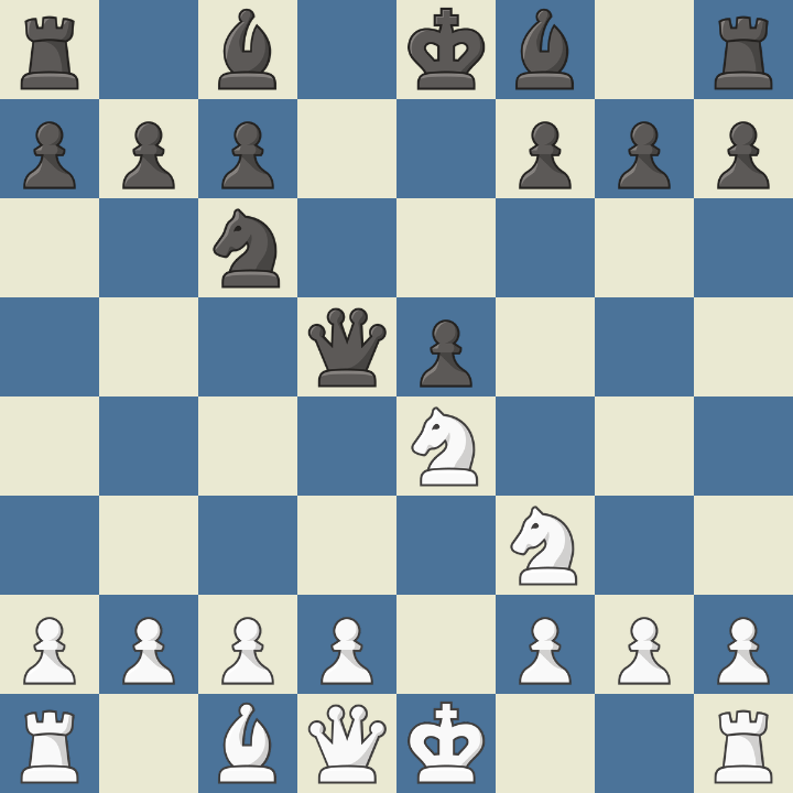
3. …Nd4

블랙번 실링 갬빗이다. 백 입장에서는 흑이 e5 폰을 내준 것 같지만 이는 함정이다. 흑의 4. …Qg5로 나이트와 g폰이 포크에 걸리기 때문이다.

파훼법은 폰을 잡는 대신 4. Nxd4 exd4로 나이트를 교환하고 캐슬링하는 것이다. 이후 흑이 5. …Bc5로 대응할 경우, 백에게 탁월한 수 6. Bxf7!!이 있다. 킹이 비숍을 잡을 경우 7. Qh5+가 흑의 어두운 비숍을 포크하기 때문에 기물 회수가 가능하다.

3. …f5

루소 갬빗이다. 흑이 f폰을 내주는 것 같지만, 백이 4. exf5를 할 경우 흑의 …e4가 나이트를 공격하게 되고, 나이트는 g칸으로 돌아오는 것밖에 살아남을 구멍이 없어 보인다. 결과적으로 백은 전개에서 뒤지게 된다.

그런데 여기에는 역공 라인이 있다. 백이 g1으로 나이트를 빼는 대신, 5. Ne4로 가는 것이다. 그러면 …Nxe4로 나이트를 잃는 것처럼 보이지만, 6. Qh5+라는 강력한 역공을 넣을 수 있다.

역공을 거는 대신 4. d4로 간단히 응수할 수도 있다. 그러면 흑이 …fxe4로 나이트를 공격하더라도 Nxe5로 전개하면 된다. 한편 흑은 f7-h5 대각선이 약점으로 남는다. (오프닝 때 f폰을 움직이지 말라는 말이 괜히 있는 것이 아니다)

---

참고자료

슥슥이 유튜브 사랑합니다

슬라보예 지젝, ｢소프트 파시즘, 인공지능, 그리고 수치심의 몰락｣

06 Jun 2025

본 글은 2024년 11월 26일에 이루어진 슬라보예 지젝의 옥스포드 강연을 번역한 것이다. 주석은 역자 주이다. 또한 섹션의 구분도 역자가 독자의 편의를 위해 넣은 것이다. 매끄러운 흐름을 위해 내용을 덧대거나 빼는 수준의 의역과 문장 재배치를 한 부분이 있다.

1. 운명론적 역사관 비판

저는 “우리가 지금 어디에 있는가”라는 질문에 대한 몇 가지 개괄적인 이야기를 하고자 합니다. — 우리는 지금 어디에 있을까요?

저는 양자역학의 개념을 빌려와서 이 사회적 · 역사적 질문에 접근하고 싶습니다. 우선 저의 기본적인 생각은, 자유주의나 마르크스주의에서 피력하는 낙관적인 역사관을 포기해야 한다는 것입니다. 이러한 역사관들은 운명론적인 특징을 가지고 있습니다. 일례로 후쿠야마_{Francis Fukuyama}는 “역사의 종말¹”을 주장했습니다. 한편 정통 마르크스주의자들은, 여러 굴곡이 있더라도 궁극적으로는 공산주의 사회가 도래할 것이라고 주장합니다. “미래는 사회주의거나 야만주의다”라고 말한 로자 룩셈부르크_{Rosa Luxemburg}처럼 운명론에서 아주 살짝 비껴난 입장도 있기는 했지요. 여담이지만, 안타깝게도 룩셈부르크는 이 점에 있어 틀렸습니다. 스탈린주의에는 둘 다 있었으니까요.

이런 운명론에 매달리기보다, 저는 다음과 같이 생각합니다. 양자역학에 따르면, 점 A에서 점 B로 이동하는 입자는 A와 B를 잇는 모든 경로를 양자 중첩 상태로 거칩니다. 우리가 관측하는 것은 그러한 중첩 상태에서 붕괴된 하나의 경로이지요. 저는 우리의 현 사회가 붕괴 전의 중첩 상태라고 생각합니다. 과연 누가 앞으로의 인류가 어디로 향할지 알겠습니까? 우리가 아는 것은 우리의 미래에 치명적인 위협들이 있다는 것뿐입니다. 환경, 전쟁, 인구 문제 등이 떠오르네요. 우리는 이러한 위협들이 어떻게 상호작용할지도 오리무중입니다. 어떤 사람들은 환경 위기가 심각해지면 전쟁은 줄어들 것이라고 생각합니다. 저는 이 점에 관해 회의적입니다.

2. 소프트 파시즘과 불량 국가

이러한 위협들에 대응하는 과정에서 어쩌면 미래에는 새로운 사회주의가 도래할지도 모릅니다. 일부 문명만이 섬처럼 고립된 형태의 세계적인 야만주의가 도래할지도 모르지요. 그러나 제가 예상하건대 — 그리고 이 예상은 저를 정말 슬프게 만듭니다 — 가장 도래할 가능성이 높은 미래는 제가 소프트 파시즘_{Soft Fascism}이라고 부르는 것입니다. 여기서 “소프트”라는 표현은 이것이 나치주의와 같은 노골적인 파시즘이 아님을 의미합니다. 제가 생각하기에 파시즘의 가장 괜찮은 정의는 “보수적인 혁명”입니다. 영리한 파시스트들은 자본주의의 활력과 빠른 발전력을 탐내면서도, 방임된 자본주의는 사회 분열을 초래한다는 사실을 알았습니다. 이 문제를 극복하기 위한 파시즘의 발상은, 강력한 국가 권력이 전통 · 종교 · 민족 등의 이데올로기를 통해 자본주의적 경제 구조를 억지로 유지해 내는 사회입니다.

제가 소프트 파시즘의 교과서적인 사례로 생각하는 국가가 있습니다. 바로 중국입니다. 두 달 전, 중국 지도자의 연설이 있었습니다. 그는 우리 세대의 젊은이들이 충분히 교육되지 않았으며 그들을 사상적으로 훈련시켜야 한다고 말했습니다. 저는 그래서 그가 늘 하던 말 — 마르크스를 읽으라는 둥, 마오를 읽으라는 둥 — 을 할 줄 알았습니다. 하지만 아니었습니다. 그가 언급한 것은 유교 전통이었습니다. 통합을 위해서는 유교 정신이 필요하다는 것이었습니다. 같은 일이 인도에서는 모디_{Narendra Modi}에 의해 행해지고 있습니다.² 극도로 야만적인 자본주의 체제가 비자본주의적인 이데올로기를 통해 유지됩니다. 저에게 물어본다면, 이것이 대다수의 국가가 봉착하게 될 미래입니다. 역사는 우리의 편에 서 있지 않습니다.

저를 염려시키는 또다른 사실은, 소위 불량 국가_{rogue state}들이 점점 많아지고 있다는 것입니다. 당황하지 마세요. 제가 말하는 “불량 국가”는 서구의 제국주의적 언어에 해당하지 않습니다.³ 제가 정의하는 “불량 국가”란, 현존하는 질서가 자기 자신의 이데올로기적 조건 속에서 스스로를 법적으로 유지할 수 없기 때문에 야만적이고 불법적인 폭력에 의존해야 하는 국가입니다.

아무래도 아이티가 가장 먼저 따오르는 사례군요. 그곳은 국가가 붕괴하여 국토의 80% 이상이 갱단에 의해 경영되고 있습니다. 하지만 굳이 아이티 같은 이례적인 사례에 집착할 필요는 없습니다. 러시아는 어떻습니까? 바그너 그룹은 전형적인 반법_半法, 불법 군사 조직으로서, 이제는 러시아 정부의 전폭적인 지지를 받아왔음이 만천하에 드러났습니다. 그럼에도 불구하고 바그너 그룹은 중앙 정부와 언제나 일정한 거리를 두었죠. 그런가 하면 이스라엘은요? 솔직해집시다. 서안 지구⁴에 정착한 이스라엘인들은 다름아닌 이스라엘의 법에 따라 범법자들입니다. 이스라엘의 비극을 잘 보여주는 사례가 있습니다. 이타마르 벤그리브는 20여년 전에 인종 범죄로 이스라엘 법정에 기소된 바 있습니다. 지금 그는 이스라엘 안보부 장관입니다. 미국도 크게 다르지 않습니다. 현재 미국에는 반이슬람주의자, 반유대주의자, 프라우드 보이즈⁵와 같은 단체들이 공존하고 있습니다. 그리고 트럼프는 그들과 거리를 두면서도 그들을 통해 사회를 조종합니다. 이들이야말로 실패한 국가들입니다. 이들은 그 자신의 이데올리기와 법적 근거만을 통해서는 질서를 지탱할 수 없는 국가들입니다.

따라서 우리는 현재의 극단적인 혼돈과 비결정성을 인지해야만 합니다. 현재의 상황이 언제까지나 이어질 수 없다는 사실은 명백합니다. 그러나 그 종착지가 어디일지는 그 어떤 의미에서도 결정된 것이 아닙니다. 다시 양자역학의 용어를 빌리자면, 우리의 중첩 상태가 어떠한 하나의 상태로 붕괴할지 전혀 알 수 없습니다. 미래가 가장 바람직한 특정 정치 형태로 나아가리라는 생각은 일종의 착시입니다.

3. 사후성

자세히 말할 시간은 없지만 저는 헤겔이 이것을 내다보았다고 생각합니다. 사후성_{retroactivity}에 관한 헤겔의 논의를 봅시다. 특정한 현실이 자리를 잡으면, 그 현실이 과거를 실질적으로 변화시키지는 않지만 사후적으로는 변화시킵니다. 다시 말해, 현재는 우리가 과거를 인지하는 방식과 과거에 부여하는 서사를 변화시킵니다. 그런 의미에서 우리는 늘 과거를 변화시키고 있습니다. 같은 주장을 마르크스에서도 발견할 수 있습니다. 마르크스는 순진한 진보주의자로 폄하되곤 하지만 — 물론 그에게 이러한 면모가 실제로 있었음은 부정할 수 없습니다 — 그에게는 다른 면모도 있습니다. 예를 들어 그의 ⟪정치경제학 비판 요강⟫에는 이런 대목이 있습니다. “인간의 해부학이 유인원의 해부학을 이해하는 열쇠인 것처럼 자본주의는 역사의 모든 단계를 해석하는 능력을 제공한다.” 마르크스의 이 대목은 놀랍도록 반-운명론적인 것입니다. 여기서 그가 말하려는 것은 “자본주의의 도래는 예정된 것이었다”와 같은 말이 아닙니다. 마르크스의 요점은 훨씬 더 정교합니다. 자본주의가 승리하고 나면, 우리는 사후적으로 역사를 해석하여 과거의 모든 사건들이 마치 자본주의를 향해 왔던 것처럼 재서술한다는 것입니다.

이러한 이유로 저는 데이비드 그레이버_{David Graeber}와 윈그로_{David Wengrow}의 연구를 — 비록 그들의 주장에 완전히 동의하지는 않지만 — 아주 높이 평가합니다. 그들은 고대 잉카 문명에서, 현대의 우리가 처한 것과 같은 중첩 상태를 포착하고자 했습니다. 잘 아시겠지만, 잉카 문명이 언제나 아이들을 희생시키는 식의 공포로 점철된 것은 아니었습니다. 잉카에서는 놀라운 수준의 지역 민주주의 체계가 작동하고 있었습니다. 어느 순간 붕괴했을 뿐이었지요. 이로부터 제가 내리는 교훈은 이것입니다. 일어나는 일들을 이해하기 위해서는, 일어날 수 있었지만 일어나지 않은 일들에 주목해야 합니다. 일어날 수 있었지만 일어나지 않은 일들은 그저 소멸하지 않습니다. 그것은 어쩌면 반동적인, 어쩌면 진보적인, 일종의 염원으로서 사회에 잔존합니다.

4. 인공지능과 인간다움

이러한 이유로 저는 우리가 “진보”를 정의하는 데 있어 매우 조심해야 한다고 생각합니다. 예를 들어 오늘날의 중요한 주제인 인공지능의 사례를 봅시다. 저는 우리가 “인공지능도 사고할 수 있게 될까?”와 같은 질문만 던져서는 인공지능의 문제에 올바르게 접근할 수 없다고 생각합니다. 물론 여기서 말하는 “사고”란 우리 인간과 같은 방식의 사고를 말합니다. 우선 이것은 우리가 답을 알지 못하는 추상적인 질문입니다. 우리는 우리와 같은 방식의 사고 가능성에 집착하지만, 완전히 새로운 형태의 정신이라든가 영혼이 생길 수도 있는 것 아니겠습니까?

대신 제가 여러분을 자극할 만한 정신분석학적 접근을 제시해 보겠습니다. “인공지능이 무엇을 할 수 있는가” — 흔히 있는 멍청한 토론 주제죠 — 라는 질문을 생각해 보면, 당연히 인공지능은 우리보다 훨씬 빠르게 계산할 수 있고, 스스로 학습할 수 있고, 자기 복제할 수 있습니다. 그러나 제 생각에는 인간에게 고유한, 그리고 인간다움의 핵심을 이루는 두 가지 특징이 있습니다.

첫째는 일상에서의 의식, 달리 말하자면 미신적 습관입니다. 개인적인 사례를 들자면 저는 손을 씻고 수도꼭지를 잠굴 때 꼭지에서 물방울이 떨어지고 있지 않다는 것을 똑똑히 보고서도 꼭지에 손을 대서 확인하곤 합니다. 정신분석학자라면 이것을 피임에 대한 무의식적 강박으로 해석할지 모르겠지만 그런 말도 안 되는 소리는 사양하겠습니다. 이것은 단적인 습관일 뿐입니다. 하지만 우리는 모두 이같은 습관을 가지고 있습니다. 제가 애거서 크리스티의 전기에서 읽은 사실인데요, 그는 목욕을 하고 나올 때마다 사과 한 알을 먹었다고 합니다. 도대체 이런 행동에 어떤 의미가 있겠습니까? 이 행동들이 가지는 의미가 있다면 그것은 외양에 불과합니다.⁶ 혹은 의미를 가지지 않는 의미라고 말할 수 있겠습니다. “이 행동의 이면에는 이러한 트라우마가 있다”라든가 “이 행동의 이면에는 이러한 무의식적 동기가 있다”라고 말하는 것은 잘못되었습니다. 애거서 크리스티가 무의식적으로 본인이 에덴 동산의 이브라고 생각했다는 말입니까? 아니죠. 이러한 텅빈 의미의 외양은 우리 인간이 노골적일 정도로 혼란스러운 삶의 무의미에 대응하는 한 가지 방식에 다름 아닙니다.

둘째로, 저는 인공지능이 결코 진정한 의미에서 욕을 할 수 없다고 생각합니다. 저에게 있어 욕은 매우 흥미로운 현상입니다. 욕은 단순히 저급한 언어가 아닙니다. 욕은 인간이 언어 안에 존재하기를 원한다는 증거입니다. 우리의 사고는 언어의 형태로 이루어지지만, 그럼에도 우리는 결코 진정한 의미에서 언어에 거주하지 않습니다. 우리가 욕을 할 때는 단순히 객관적 사건에 대한 불만족을 표출하는 것이 아닙니다. 욕은 그것을 언어로 형성할 수 없는 데에서 오는 분노의 표출입니다. 일례로 십자가에 매달린 예수를 떠올려 보세요. 저는 아무리 예수라고 해도 죽어가면서 욕을 했을 것이라고 생각합니다. 다소 어이없는 생각이긴 하지만, “와 시발…”이라고 중얼거렸을 수도 있지 않을까요? 제 요점은, 언어 안에 완전히 존재할 수 없을 때 느끼는 수치심이야말로 인간다움을 구성하는 본질 중 하나라는 것입니다.

5. 수치심의 몰락

이제 또다른, 어쩌면 놀랍게 들릴 수도 있는 이야기로 마무리를 짓겠습니다. 오늘날 저를 정말로 슬프게 만드는 것은 뻔뻔함_{shamelessness}의 폭증입니다. 10년 전까지만 해도 공적인 장소에서 말하는 것이 불가능했던 말들이 이제는 공공연하게 이루어집니다. 단순히 도널드 트럼프나 보리스 존슨과 같은 뻔한 사례들을 말하려는 것이 아닙니다. 저는 단연코 반유대주의자가 아니지만 — 저는 이스라엘의 입장도 고려하려 합니다 — 최근에 이스라엘에서 일어난 두 가지 일은 저를 충격에 빠뜨렸습니다. 8월에 이스라엘 의회 케네셋에서 논쟁이 있었습니다. 먼저 배경을 말씀드리겠습니다. 예루살렘의 남쪽에 있는 하마스 수용소에서는 간수들이 수감자들을 매우 잔혹하게 다루고 있었습니다. 영상 자료도 유출되었기 때문에 부정할 수 없는 사실이지요. 바늘로 뒤덮인 커다란 철제 막대기를 항문에 쑤셔 넣는 등의 고문으로 인해 많은 수감자가 과다출혈로 사망했습니다. 물론 저는 중립을 지키고 싶기 때문에 하마스 측에서는 무슨 고문을 하고 있을지 누가 아냐는 단서를 남겨두겠습니다. 하지만 저를 정말 슬프게 만드는 것은, 케네셋의 논쟁에서 지배적이었던 의견이 간수들의 잘못을 따지는 것이 아닌, 가혹행위를 한 간수들이 기소되었다는 사실을 치욕으로 여기는 의견이었다는 것입니다. 하마스는 인간도 아니기에 그들에게는 무슨 짓을 해도 괜찮다는 것이었죠. 저는 이런 솔직함보다는 위선이 낫다고 생각합니다.

이제 두 번째 사건을 말해 보겠습니다. 엘리란 미즈라히라는 한 정직하고 올바른 이스라엘 병사가 있었습니다. 가자에서 복무할 당시 그는 끔찍한 명령을 받았습니다. 생사 여부를 따지지 말고 수백 명의 팔레스타인을 트랙터로 깔아뭉개라는 명령이었습니다. 그는 명령을 이행했지만 이후 극심한 혼란에 살다가 이내 자살했습니다. 미즈라히는 윤리적 고결함을 가지고 있었던 것이지요. 그러나 이를 본 이스라엘 방위군의 심리전문가들은 어떻게 병사들을 훈련시켜야 그들이 윤리적 딜레마를 느끼지 않도록 할 수 있을지를 연구하기 시작했습니다. 이것이 제가 말하는 “뻔뻔함”입니다.

그렇다면 이제 정말로 결론을 내리겠습니다. 저에게 무척이나 흥미로운 것은, 저의 스승이라고 부를 수 있을 자크 라캉의 견해입니다. 그는 69-70년에 정신분석학의 다른 측면에 대한 세미나를 진행했었는데요, 그 세미나는 68혁명에 대한 그의 반응이기도 했습니다. 세미나에서 라캉은 학생 저항을 지지하는 대신 이렇게 말했습니다. “당신들에게 결여되어 있는 것은 수치심이다.” 라캉에 따르면, 자유방임적인 오늘날의 사회에서 정신분석학의 궁극적인 목표는 아버지의 억압을 몰아내거나 성적 환상을 실현하는 것이 아닙니다. 오히려 수치의 결여, 그리고 그것이 야기하는 보편적인 도착증_perversion이 주제입니다.

도착증은 히스테리아에 비해 훨씬 덜 전복적입니다. 정신분석학에 대해 조금 들은 바가 있다면 아시겠지만, 이 두 증세는 성별과 결부되곤 합니다. 남성 쇼비니즘의 일환입니다만, 요지는 여성은 히스테리적이라 불평을 하면서도 은밀하게 새로운 주인에게 지배받기를 원하고, 남성은 도착적이라서 자신의 꿈을 시행에 옮기기에 급급하다는 것입니다. 하지만 일찍이 프로이트는 알고 있었습니다. 도착증보다 무의식이 더 억압받는 곳은 없으며, 모든 위대한 일은 히스테리아를 통해 발생한다는 사실을 말입니다. 저는 이것이 오늘날의 우리를 위한 교훈이라고 생각합니다.⁷

제가 젊었을 때 저와 친구들은 촌스러운 좌파였습니다. 우리는 권력자들이 위엄을 지니고 있다고 생각했고, 우리 자신은 온갖 상스러운 손짓과 더러운 말을 주고받았지요. 하지만 이제는 압니다. 권력을 가진 저들이야말로 우리가 상상했던 것 이상으로 상스러운 자들입니다. 지난 선거 때 우리는 완전히 틀렸었습니다. 민주당은 아무것도 배우지 못한 것이죠. 트럼프가 거짓말을 했음이 밝혀졌을 때 민주당은 그의 약점을 잡았다고 생각했어요. 하지만 아니었지요! 오히려 그에게 도움이 됐습니다. 트럼프의 천박함과 거짓말은 그의 정체성을 이룹니다. 사람들은 바로 그 이유에서 그를 사랑했던 것이지요. 따라서 자유방임적인 오늘날의 시대에서 우리가 물어야 하는 질문은 이것입니다. 어떻게 가장 기본적인 수치심의 감각을 되살릴 것인가?

감사합니다.

---

Slavoj Žižek, "Soft Fascism, Artificial Intelligence, and Shamelessness"

06 Jun 2025

This post is originally a Korean translation of Slavoj Žižek’s Oxford lecture, so there is no separate English version. However, the following personal observation from the original post is reproduced here.

Psychoanalytically, Perversion is a manifestation of subconscious positivity while hysteria is a manifestation of subconscious negativity. Positivity encompasses concepts such as freedom, laissez-faire, liveliness, and activity, while negativity encompasses concepts such as repression, constraint, prohibition, and passivity. In this lecture, Žižek appears to subsume “soft fascism” — the pathological fusion of ideology and capitalism, — artificial intelligence, and the rise of Shamelessness under the category of perversion, namely the uncontrolled manifestation of positivity.

왜 연속함수의 위상적 정의는 “반대”인가?

02 Jun 2025

정의. 두 위상공간 $X, Y$에 대해 사상 $f: X \to Y$가 연속이라는 것은, $V \subseteq Y$가 열린 집합이라면 $f^{-1}[V] \subseteq X$ 또한 열린 집합이라는 것이다.

위상수학을 처음 수강하는 학생들은 위 정의에서 혼란을 겪는다. 직관적으로는 “$U \subseteq X$가 열린 집합이라면 $f[U] \subseteq V$ 또한 열린 집합인 사상”이라는 정의가 자연스러운데, 실제 정의는 이와 반대이기 때문이다. 이러한 직관의 “근거”는 대충 다음과 같을 것이다.

1. 엡실론-델타 논법

엡실론-델타 논법에 따르면 $f: X \to Y$가 연속이라는 것은 다음과 같다.

\[\forall \epsilon > 0 \; \exists \delta > 0 : |x - y| < \delta \rightarrow |f(x) - f(y)| < \epsilon\]

위 논리식을 보면 조건부에 $x, y \in X$가 있고 결론부에 $f(x), f(y) \in Y$가 있다. 따라서 연속함수의 위상적 정의 또한 조건부에 $U \subseteq X$가 있고 결론부에 $f[U] \subseteq Y$가 있는 것이 자연스러워 보인다.

2. 열린 집합에 대한 직관

처음 위상수학을 배울 때, 열린 집합을 “서로 가까운 점들의 모임”으로 생각하곤 한다. 즉, $U$가 열린 집합이라는 것은 $x, y \in U$라면 $x, y$가 “가깝다”는 것이다. 그렇다면 연속함수는 “가까운 점들을 가까운 점들로 사상시키는 함수”이므로, 열린 집합을 열린 집합으로 사상시키는 함수로 정의하는 것이 자연스러워 보인다.

그러나 위 두 “근거”는 매우 잘못되었다.

3. “엡실론-델타 논법” 근거가 잘못된 이유

$\rightarrow$만을 기준으로 왼쪽이 조건부, 오른쪽이 결론부로 판단하는 것은 오해를 낳기 딱 좋다. 왜냐하면 여기서는 양화사 또한 고려해야 하기 때문이다. 엡실론-델타 논법의 양화사 부분을 언어적으로 읽으면 “임의의 양수 $\epsilon$에 대해, 어떤 양수 $\delta$가 존재한다” 이다. 다른 말로 하자면, U$\epsilon$이 양수라면, 어떤 양수 $\delta$가 존재한다” 이다.

그리고 $\epsilon$과 유관한 공간은 $X$가 아닌 $Y$이다. 즉, $\epsilon$에 대한 서술, 그리고 그에 부수되는 $Y$에 대한 서술이 해당 논리식에서 가장 일차적인 조건부인 것이다. 따라서 위상적 정의에서 $V \subseteq Y$가 조건부에 있는 것은 이상한 일이 아니다.

4. “열린 집합에 대한 직관” 근거가 잘못된 이유

편의를 위해 $x$와 $y$가 “가깝다”는 것을 $x \sim y$로 표기하자. “열린 집합에 대한 직관” 근거는 다음의 잘못된 직관에 기반한다.

열린 집합에 대한 잘못된 직관. $x \in U$에 대해, $y \in U$라면 $x \sim y$이다.

이는 다음과 같이 수정해야 한다.

열린 집합에 대한 올바른 직관. $x \in U$에 대해, $x \sim y$라면 $y \in U$이다.

조금만 생각해 보면 이는 당연하다. 일례로 실수 전체의 집합 $\mathbb{R}$은 열린 집합이다. 그렇다면 임의의 두 실수는 언제나 “가까운” 것인가? 그건 말도 안 된다. 반대 경우를 보면, $\lbrace 0 \rbrace $은 열린 집합이 아니지만 $x, y \in \lbrace 0 \rbrace $일 때 $x = y$이므로 $x$와 $y$는 최대한으로 “가깝다”. 따라서 “잘못된 직관”에 따르면 $\lbrace 0 \rbrace $은 열린 집합이다.

반면 “올바른 직관”으로 보면 $\mathbb{R}$은 열린 집합이고 $\lbrace 0 \rbrace $은 열린 집합이 아닌 것이 분명하게 드러난다. $x \in \mathbb{R}$일 때, $x$와 “가까운” 실수 $y$는 자명하게 $\mathbb{R}$에 포함된다. 한편 $\lbrace 0 \rbrace $은 $0$의 “바로 곁”에 있는 실수들을 포함하고 있지 않으므로 열린 집합이 아니다.

또한 “올바른 직관”으로 보면 연속함수의 위상적 정의가 “뒤집혀야” 하는 이유 또한 분명하다. 먼저 연속함수는 다음과 같이 직관적으로 이해할 수 있다.

연속함수에 대한 올바른 직관. $x \sim y$라면 $f(x) \sim f(y)$이다.

이제 위의 “직관”과 연속함수의 위상적 정의가 동치임을 보이자.

직관적 정의 => 위상적 정의

$f$가 “직관적으로 연속”일 때, 열린 집합 $V$에 대해 $U = f^{-1}[V]$가 열린 집합임을 보이자. $x \in U$, $x \sim y$라고 하자. $f$가 연속이므로 $f(x) \sim f(y)$이다. 그리고 $V$가 열린 집합이며 $f(x) \in V$이므로 $f(y) \in V$이다. 따라서 $y \in U$이다. □

위상적 정의 => 직관적 정의

$f$가 “위상적으로 연속”일 때, $x \sim y$라면 $f(x) \sim f(y)$임을 보이자. $V$가 $f(x)$와 “가까운” 점들만을 포함하는 집합이라고 하자. $V$는 열린 집합이다. 왜냐하면 $z \in V$이고 $z \sim w$일 때, $V$의 정의에 의해 $f(x) \sim z$이므로 ~추이성에 의해~ $f(x) \sim w$, 즉 $w \in V$이기 때문이다. 그리고 $U = f^{-1}[V]$가 $x$를 포함하는 열린 집합이므로 $y \in U$이다. 따라서 $f(y) \in V$, 즉 $f(x) \sim f(y)$이다. ■

물론 위의 논의는 엄밀하게 정의되지 않은 관계 $\sim$을 사용하기 때문에 조금 석연찮기는 하다. 그러나 필자는 $\sim$을 사용하여 열린 집합과 연속성을 이해하는 것이 위상수학을 처음 공부하는 데 있어 유용한 길잡이가 되어준다고 생각한다. 덧붙이자면, 비표준 해석학을 사용하면 $x \sim y$를 $|x - y| = \epsilon$으로 엄밀하게 정의할 수 있다. 이에 관해서는 나중에 기회가 되면 이야기해 보겠다.