디멘의 블로그 Dimen's Blog
기수 연산
16 Sep 2025이 글에서 모든 집합과 기수는 무한하다.
1. 기수 덧셈
기수 산술cardinal arithmetics을 다룰 때에는 각 연산의 정의를 정확히 아는 것이 중요하다. 정의와 정리를 혼동하기가 쉽기 때문이다. 먼저 기수 덧셈부터 보자.
정의. $A, B$가 각각 기수가 $\kappa, \lambda$인 서로소 집합이라고 하자. $\kappa + \lambda$를 $|A \cup B |$로 정의한다.
정리. 기수의 유한 덧셈은 교환법칙과 결합법칙을 만족한다.
위 정의가 well-defined임을 보이기 위해서는 $\kappa + \lambda$가 $A, B$의 선택에 의존적이지 않음을 보여야 한다. 이는 ZF에서 쉽게 증명 가능하다. 또한 유한한 기수 덧셈은 그저 최대 기수를 구하는 것이기 때문에 계산하기가 상당히 용이하다.
정리.
\[\kappa + \lambda = \mathrm{max}(\kappa, \lambda)\]
증명. “2. 기수 곱셈”의 보조정리와 칸토어-베른슈타인 정리에 의해, $\aleph_\alpha = \aleph_\alpha + \aleph_\alpha$이다. 따라서 $|A| \leq |B|$라면 $|B| \leq |A + B| \leq |B + B| = |B|$이다. ■
기수 덧셈의 정의를 무한한 경우로 확장하면,
정의. 각 $i \in I$에 대해 $A_i$가 기수 $\kappa_i$인 쌍으로 서로소인 집합족 $\lbrace A_i \rbrace $가 주어졌을 때, 다음과 같이 정의한다.
\[\sum_{i \in I} \kappa_i = \left| \bigcup_{i \in I}A_i \right|\]
유의할 점은, 위 정의가 well-defined임을 보이는 데는 선택 공리가 필요하다는 점이다. 각 $i \in I$에 대해 일대일 대응 $A_i \to \kappa_i$을 선택할 수 있어야 하기 때문이다. 그래서 기수 산술을 다룰 때에는 거의 언제나 선택 공리를 전제한다.
$\kappa + \lambda = \mathrm{max}(\kappa, \lambda)$ 관계식으로부터 다음의 관계식을 유도하고 싶을 수 있지만, 성립하는 식이 아님에 주의해야 한다.
주의. $\sum_{i \in I} \kappa_i = \sup \kappa_i$는 일반적으로 성립하지 않는다.
2. 기수 곱셈
그렇다면 무한한 기수 덧셈은 어떻게 계산해야 할까? 이를 알아보기 위해, 먼저 기수 곱셈을 정의하자.
정의. $A, B$가 각각 기수가 $\kappa, \lambda$인 집합이라고 하자. $\kappa \cdot \lambda$를 $| A \times B|$로 정의한다.
정리. 기수의 유한 곱셈은 교환법칙과 결합법칙을 만족한다.
아주 용이하게도 유한 기수 곱셈의 계산은 유한 기수 덧셈의 계산과 같다.
정리.
\[\kappa \cdot \lambda = \mathrm{max}(\kappa, \lambda)\]
증명. 다음의 보조정리로부터 따라 나온다. ■
보조정리. 임의의 $\alpha \in \mathrm{Ord}$에 대해, $\aleph_\alpha \cdot \aleph_\alpha = \aleph_\alpha$
증명 개요는 다음과 같다. 임의의 $\alpha \in \mathrm{Ord}$에 대해, 다음과 같이 정의된 순서 $\prec$가 $\omega_\alpha \times \omega_\alpha$의 정렬 순서임을 보인다. $\hat{x} = \mathrm{max}(x_1, x_2), \hat{y} = \mathrm{max}(y_1, y_2)$일 때,
\[(x_1, x_2) \prec (y_1, y_2) \iff \begin{cases} \hat{x} < \hat{y}\\ x_1 < y_1 \quad (\text{if }\hat{x} < \hat{y}) \\ x_2 < y_2 \quad (\text{if }\hat{x} < \hat{y}, x_1 = y_1) \\ \end{cases}\]즉, $\prec$은 최댓값 우선 후 사전식 순서이다. 초한귀납법에 따라 모든 $\beta < \alpha$에 대해 $\aleph_\beta \cdot \aleph_\beta = \aleph_\beta$일 때 $\aleph_\alpha \cdot \aleph_\alpha = \aleph_\alpha$임을 보인다. 이를 위해 $(\omega_\alpha \times \omega_\alpha, \prec)$의 순서형order type이 $\omega_\alpha$를 넘지 않음을 보이면 된다. 이를 위해 임의의 $(\gamma_1, \gamma_2) \in \omega_\alpha \times \omega_\alpha$에 대해
\[X = \{ (\xi_1, \xi_2) : (\xi_1, \xi_2) \prec (\gamma_1, \gamma_2) \}\]라면 $|X| < \aleph_\alpha$임을 보이면 된다. $\gamma = \mathrm{max}(\gamma_1, \gamma_2) + 1$이라고 하자. $\omega_\alpha$는 극한 서수이므로 $\gamma \in \omega_\alpha$이며, 따라서 $|\gamma| = \aleph_\delta \; (\delta < \alpha)$이다. 한편으로 $X \subseteq \gamma \times \gamma$이므로 $|X| \leq \aleph_\delta \cdot \aleph_\delta$이며 이는 귀납 가정에 의해 $\aleph_\delta$이다. ■
기수 곱셈의 정의는 기수 덧셈과 아무 관련이 없다. 즉, 기수 곱셈의 정의에는 “$\kappa$를 $\lambda$번 더한다”와 같은 의미가 없다. 그럼에도 다음 정리에 의해 기수 곱셈을 기수 덧셈과 연관지을 수 있다.
정리.
\[\sum_{i \in I} \kappa = |I| \cdot \kappa\]
증명. $\lbrace A_i \rbrace $가 쌍으로 서로소이며 $|A_i| = \kappa$인 집합족이라고 하자. 좌변은 $\bigcup_{i \in I} A_i$의 기수이고, 우변은 $I \times A$의 기수이다 $(|A| = \kappa)$. 선택 공리에 의해 각 $i \in I$에 대해 일대일 대응 $f_i : A_i \to A$를 정의할 수 있다. 다음의 대응 $f: \bigcup_{i \in I} A_i \to I \times A$을 정의하자.
\[f(x) = (i, f_i(x)) \quad (\text{if } x \in A_i)\]위 함수가 일대일 대응임은 쉽게 확인할 수 있다. 따라서 (좌변) = (우변)이다. ■
이로부터 앞선 언급한 “주의”에 해당되는 올바른 관계식을 증명할 수 있다.
정리.
\[\sum_{i \in I} \kappa_i = |I| \cdot \sup \kappa_i\]
증명. $\kappa = \sup \lbrace \kappa_i : i \in I \rbrace $라고 하고, 좌변을 $L$, 우변을 $R$이라고 하자. 앞선 정리에 의해 $|I| \cdot \kappa = \sum_{i \in I} \kappa$이고 $\kappa_i \leq \kappa$이므로 $L ≤ R$이다. 반대로, $| I | = \sum_{i \in I} 1 \leq L$이고, $\kappa = \sup \kappa_i \leq L$이다. 글 하단의 보조정리에 의해 $L = L \cdot L$이므로 $L \geq | I | \cdot \kappa = R$이다. 따라서 칸토어-베른슈타인 정리에 의해 $L = R$이다. (이 증명에는 선택 공리가 암시적으로 많이 사용되었으니 관심 있는 독자는 생략된 논증을 자세히 써 봐도 좋을 것이다) ■
이제 기수 곱셈도 무한 경우로 일반화하자.
정의. 각 $i \in I$에 대해 $A_i$가 기수 $\kappa_i$인 집합족 $\lbrace A_i \rbrace $가 주어졌을 때, 다음과 같이 정의한다.
\[\prod_{i \in I} \kappa_i = \left| \prod_{i \in I}A_i \right|\]
기수 곱셈을 계산할 때 쾨니히 정리König’s Theorem가 유용하게 사용될 수 있다.
쾨니히 정리. 인덱스 집합 $I$에 대해 $\kappa_i < \lambda_i$라고 하자. 다음이 성립한다.
\[\sum \kappa_i < \prod \lambda_i\]
당연한 거 아니냐고 생각할 수 있겠지만, 일반적으로 1, 2는 고사하고 3도 성립하지 않는다는 사실에 유의하라.
- $\kappa_i < \lambda_i$라면 $\sum \kappa_i < \sum \lambda_i$
- $\kappa_i < \lambda_i$라면 $\prod \kappa_i < \prod \lambda_i$
- $\kappa_i \leq \lambda_i$일 때 $\sum \kappa_i < \prod \lambda_i$
물론 1, 2, 3에서 결론부의 부등호를 $<$에서 $\leq$로 약화하면 모두 성립한다. 쾨니히 정리의 특징은 결론부가 엄격한 부등호라는 것이다.
증명. $\lbrace A_i \rbrace , \lbrace B_i \rbrace $가 각각 기수가 $\kappa_i, \lambda_i$인 (쌍으로 서로소인) 집합들의 모임이라고 하자. 귀류법에 따라, $f: \prod B_i \to \cup A_i$인 단사함수가 존재한다고 하자. 임의의 $i \in I$에 대해, $f$의 단사성으로부터 $|f^{-1}(A_i)| = |A_i|$이다. 그런데 $|A_i| < |B_i|$이므로 $\pi_i (f^{-1}(A_i)) \subset B_i$는 $B_i$보다 크기가 엄격히 작으며, 이에 따라 $b_i \in B_i \setminus \pi_i (f^{-1}(A_i))$가 존재한다. 각 $i$에 대해 그러한 $b_i$를 고른 뒤, $b = (b_i)_{i \in I}$를 생각하면, 임의의 $i \in I$에 대해 $\pi_i(b) = b_i$이므로 $f(b) \notin \cup A_i$가 되어 모순이다. ■
3. 기수 지수
정의. $A, B$가 각각 기수가 $\kappa, \lambda$인 집합이라고 하자. $\kappa^\lambda$를 $|A^B |$로 정의한다. ($A^B$는 $B$에서 $A$로 가는 함수들의 집합이다)
기수 곱셈의 경우와 마찬가지로, 비록 기수 지수의 정의는 기수 곱셈과 아무 관련이 없지만, 다음 정리에 의해 둘 사이에 다리를 놓을 수 있다.
정리.
\[\prod_{i \in I} \kappa = \kappa^{|I|}\]
또한 기수 지수는 일반적인 지수의 여러 좋은 성질을 공유한다.
정리. 기수의 지수 연산은 지수법칙을 만족한다. 즉,
- $\kappa^{\lambda + \mu} = \kappa^\lambda \cdot \kappa^\mu$
- $(\kappa^\lambda)^\mu = \kappa^{\lambda \cdot \mu}$
- $(\kappa \cdot \lambda)^{\mu} = \kappa^\mu \cdot \lambda^\mu$
그럼에도 기수 지수를 정확히 계산하기란 굉장히 까다로운데, 일반화된 연속체 가설Generalized Continuum Hypothesis을 전제하지 않으면 얻을 수 있는 결과가 제한적이기 때문이다. 우선 일반화된 연속체 가설 없이 증명할 수 있는 정리들을 보자.
정리.
- $2^{\aleph_\alpha} > \aleph_\alpha$
- $\alpha \leq \beta \implies \kappa^{\aleph_\alpha} \leq \kappa^{\aleph_\beta}$
- $\mathrm{cf}(\kappa^{\aleph_\alpha}) > \aleph_\alpha$
$\mathrm{cf}(\kappa) \leq \kappa$이므로 3이 1을 함의한다는 사실에 주목하라.
증명. 1은 칸토어의 정리이고, 2는 선택 공리를 사용하면 자명하다. 3의 증명은 쾨니히 정리를 사용한다. $\mathrm{cf}(\kappa^{\aleph_\alpha}) = \aleph_\lambda$라고 하자. $\mathrm{cf}$의 정의에 의해 $\xi_i < \kappa^{\aleph_\alpha}$이며 $\sum_{i < \omega_\lambda} \xi_i = \kappa^{\aleph_\alpha}$을 만족하는 $\lbrace \xi_i \rbrace _{i < \omega_\lambda}$가 존재한다. 쾨니히 정리에 의해 다음이 성립한다.
\[\kappa^{\aleph_\alpha} = \sum_{i < \omega_\lambda} \xi_i < \prod_{i < \omega_\lambda} \kappa^{\aleph_\alpha} = \kappa^{\aleph_\alpha \cdot \aleph_\lambda}\]그런데 만약 $\aleph_\lambda = \aleph_\alpha$라면 $\kappa^{\aleph_\alpha \cdot \aleph_\lambda} = \kappa^{\aleph_\alpha}$이므로 $<$가 성립하지 않는다. 따라서 $\aleph_\lambda > \aleph_\alpha$이다. ■
다음의 두 정리는 특히 유용하다.
정리.
\[\aleph_\alpha^{\aleph_\beta} = \begin{cases} 2^{\aleph_\beta} & (\aleph_\alpha \leq \aleph_\beta) \\ \mathrm{card} \{ A \subseteq \omega_\alpha : |A| = \aleph_\beta \} & (\aleph_\beta < \aleph_\alpha) \end{cases}\]
증명. $\aleph_\alpha \leq \aleph_\beta$인 경우의 증명은 다음과 같다.
\[2^{\aleph_\beta} \leq \aleph_\alpha^{\aleph_\beta} \leq (2^{\aleph_\alpha})^{\aleph_\beta} = 2^{\aleph_\alpha \cdot \aleph_\beta} = 2^{\aleph_\beta}\]$\aleph_\alpha > \aleph_\beta$인 경우를 증명하자. 좌변의 집합을 $S$라고 하자. 각 $S$의 원소는 $\aleph_\beta$에서 $\aleph_\alpha$로 가는 단사함수로 생각할 수 있으므로 $|S| \leq {\aleph_\alpha}^{\aleph_\beta}$이다. 역방향을 보이기 위해 먼저 $\aleph_\beta < \aleph_\alpha$이므로 $\aleph_\alpha = \aleph_\beta \cdot \aleph_\alpha$임을 관찰하자. 따라서,
\[|S| = |T| \quad \text{where} \quad T = \{ A \subseteq \omega_\beta \times \omega_\alpha : |A| = \aleph_\beta \}\]그런데 $T$의 각 원소는 $\omega_\alpha$에서 중복을 허용하고 $\aleph_\beta$개의 원소를 뽑는 경우의 수로 생각될 수 있다. 이는 $T$에서 ${\aleph_\alpha}^{\aleph_\beta}$로 가는 전사 관계를 정의한다. 따라서 ${\aleph_\alpha}^{\aleph_\beta} = |S|$이다. ■
이의 따름정리는 하우스도르프 정리이다.
하우스도르프 정리.
\[\aleph_{\alpha+1}^{\aleph_\beta} = \aleph_\alpha^{\aleph_\beta} \cdot \aleph_{\alpha + 1}\]
증명. $\beta > \alpha$라면 앞선 정리에 의해 정리가 자명하게 성립한다. 따라서 $\beta \leq \alpha$라고 하자. $\aleph_{\alpha+1}^{\aleph_\beta} \geq \aleph_\alpha^{\aleph_\beta}, \aleph_{\alpha + 1}$이므로 $\geq$ 방향은 자명하게 성립한다. 따라서 $\leq$ 방향을 보이면 충분하다.
$\aleph_{\alpha + 1}$은 계승자 기수successor cardinal이므로 정칙regular이며, 이에 따라 $\aleph_\beta < \mathrm{cf}(\aleph_{\alpha + 1})$이다. 따라서 $f \in \omega_\alpha^{\omega_\beta}$는 상계를 가진다. 즉,
\[\aleph_{\alpha+1}^{\aleph_\beta} = \bigcup_{\gamma < \omega_{\alpha + 1}} \gamma^{\omega_\beta}\]여기서 각 $\gamma$는 기수가 $\aleph_\alpha$ 이하이다. 따라서 다음이 성립한다.
\[\aleph_{\alpha+1}^{\aleph_\beta} \leq \sum_{\gamma < \omega_{\alpha + 1}} |\gamma|^{\aleph_\beta} \leq \sum_{\gamma < \omega_{\alpha + 1}} {\aleph_\alpha}^{\aleph_\beta} = {\aleph_\alpha}^{\aleph_\beta} \cdot \aleph_{\alpha + 1} \quad \blacksquare\]4. 일반화된 연속체 가설 하에서
일반화된 연속체 가설을 전제하면 훨씬 더 강력한 결과들을 증명할 수 있다.
정리. $\aleph_\alpha$가 정칙 기수인 경우, 다음이 성립한다.
\[\aleph_\alpha^{\aleph_\beta} = \begin{cases} \aleph_{\beta + 1} & \aleph_\alpha \leq \aleph_\beta \\ \aleph_{\alpha} & \aleph_\beta < \aleph_\alpha \end{cases}\]
증명. $\aleph_\alpha \leq \aleph_\beta$인 경우 $\aleph_\alpha^{\aleph_\beta} = 2^{\aleph_\beta}$이므로 GCH에 의해 성립한다. $\aleph_\alpha > \aleph_\beta$인 경우,
\[\aleph_\alpha^{\aleph_\beta} = |S| \quad \text{where} S = \{ A \subseteq \omega_\alpha : |A| = \aleph_\beta \}\]이다. $\aleph_\alpha$가 정칙이므로 $S$의 각 원소는 유계이다. 따라서,
\[S \subseteq \bigcup_{\lambda \in \omega_\alpha} \mathcal{P}(\lambda)\]이다. 임의의 $\lambda \in \omega_\alpha$에 대해 $|\lambda| = \aleph_\delta$라고 하면, $\aleph_\delta < \aleph_\alpha$이므로 $2^{|\lambda|} = \aleph_{\delta + 1} < \aleph_\alpha$이다. 따라서 다음이 성립한다.
\[\begin{align} |S| &\leq \sum_{\lambda \in \omega_\alpha} 2^{|\lambda} \\ &\leq \sum_{\lambda \in \omega_\alpha} \aleph_\alpha \\ &= \aleph_\alpha \cdot \aleph_\alpha = \aleph_\alpha \quad \blacksquare \end{align}\]정리. $\aleph_\alpha$가 특이 기수인 경우, 다음이 성립한다.
\[\aleph_\alpha^{\aleph_\beta} = \begin{cases} \aleph_{\beta + 1} & \aleph_\alpha \leq \aleph_\beta \\ \aleph_{\alpha + 1} & \mathrm{cf}(\aleph_\alpha) \leq \aleph_\beta < \aleph_\alpha \\ \aleph_{\alpha} & \aleph_\beta < \mathrm{cf}(\aleph_\alpha) \end{cases}\]
증명. 첫 번째 경우와 세 번째 경우는 이전 정리의 증명과 거의 같으므로, 두 번째 경우만 살펴보자. 다음이 성립한다.
\[\aleph_\alpha \leq \aleph_\alpha^{\aleph_\beta} \leq \aleph_\alpha^{\aleph_\alpha} = 2^{\aleph_\alpha} = \aleph_{\alpha+1}\]따라서 $\aleph_\alpha < \aleph_\alpha^{\aleph_\beta}$임을 보이면 충분하다. 만약 $\aleph_\alpha = \aleph_\alpha^{\aleph_\beta}$라면 $\mathrm{cf}(\aleph_\alpha) = \mathrm{cf}(\aleph_\alpha^{\aleph_\beta}) > \aleph_\beta$인데, 가정에 의해 $\mathrm{cf}(\aleph_\alpha) \leq \aleph_\beta$이므로 모순이다. ■
Cardinal Arithmetic
16 Sep 2025This post was originally written in Korean, and has been machine translated into English. It may contain minor errors or unnatural expressions. Proofreading will be done in the near future.
In this article, all sets and cardinals are infinite.
1. Cardinal Addition
When dealing with cardinal arithmetic, it is important to know the precise definitions of each operation. It is easy to confuse definitions with theorems. Let us begin with cardinal addition.
Definition. Let $A, B$ be disjoint sets with cardinalities $\kappa, \lambda$ respectively. Define $\kappa + \lambda$ as $|A \cup B |$.
Theorem. Finite cardinal addition satisfies the commutative and associative laws.
To show that the above definition is well-defined, we must prove that $\kappa + \lambda$ does not depend on the choice of $A, B$. This is easily provable in ZF. Moreover, finite cardinal addition is merely finding the maximum cardinal, making it quite easy to compute.
Theorem.
\[\kappa + \lambda = \mathrm{max}(\kappa, \lambda)\]
Proof. By the lemma in “2. Cardinal Multiplication” and the Cantor-Bernstein theorem, $\aleph_\alpha = \aleph_\alpha + \aleph_\alpha$. Therefore, if $|A| \leq |B|$, then $|B| \leq |A + B| \leq |B + B| = |B|$. ■
Extending the definition of cardinal addition to the infinite case,
Definition. Given a family of pairwise disjoint sets $\lbrace A_i \rbrace $ where each $A_i$ has cardinality $\kappa_i$ for $i \in I$, we define:
\[\sum_{i \in I} \kappa_i = \left| \bigcup_{i \in I}A_i \right|\]
Note that proving this definition is well-defined requires the axiom of choice. For each $i \in I$, we must be able to choose a bijection $A_i \to \kappa_i$. Therefore, when dealing with cardinal arithmetic, the axiom of choice is almost always presupposed.
From the relation $\kappa + \lambda = \mathrm{max}(\kappa, \lambda)$, one might wish to derive the following relation, but note that this is not a valid equation.
Warning. $\sum_{i \in I} \kappa_i = \sup \kappa_i$ does not hold in general.
2. Cardinal Multiplication
How then should we compute infinite cardinal addition? To understand this, let us first define cardinal multiplication.
Definition. Let $A, B$ be sets with cardinalities $\kappa, \lambda$ respectively. Define $\kappa \cdot \lambda$ as $| A \times B|$.
Theorem. Finite cardinal multiplication satisfies the commutative and associative laws.
Very conveniently, the computation of finite cardinal multiplication is the same as that of finite cardinal addition.
Theorem.
\[\kappa \cdot \lambda = \mathrm{max}(\kappa, \lambda)\]
Proof. This follows from the lemma below. ■
Lemma. For any $\alpha \in \mathrm{Ord}$, $\aleph_\alpha \cdot \aleph_\alpha = \aleph_\alpha$
The proof outline is as follows. For any $\alpha \in \mathrm{Ord}$, we show that the order $\prec$ defined as follows is a well-ordering of $\omega_\alpha \times \omega_\alpha$. When $\hat{x} = \mathrm{max}(x_1, x_2), \hat{y} = \mathrm{max}(y_1, y_2)$,
\[(x_1, x_2) \prec (y_1, y_2) \iff \begin{cases} \hat{x} < \hat{y}\\ x_1 < y_1 \quad (\text{if }\hat{x} < \hat{y}) \\ x_2 < y_2 \quad (\text{if }\hat{x} < \hat{y}, x_1 = y_1) \\ \end{cases}\]That is, $\prec$ is the maximum-first then lexicographic order. By transfinite induction, we show that $\aleph_\alpha \cdot \aleph_\alpha = \aleph_\alpha$ when $\aleph_\beta \cdot \aleph_\beta = \aleph_\beta$ for all $\beta < \alpha$. For this, it suffices to show that the order type of $(\omega_\alpha \times \omega_\alpha, \prec)$ does not exceed $\omega_\alpha$. We need to show that for any $(\gamma_1, \gamma_2) \in \omega_\alpha \times \omega_\alpha$,
\[X = \{ (\xi_1, \xi_2) : (\xi_1, \xi_2) \prec (\gamma_1, \gamma_2) \}\]satisfies $|X| < \aleph_\alpha$. Let $\gamma = \mathrm{max}(\gamma_1, \gamma_2) + 1$. Since $\omega_\alpha$ is a limit ordinal, $\gamma \in \omega_\alpha$, and therefore $|\gamma| = \aleph_\delta$ for some $\delta < \alpha$. On the other hand, $X \subseteq \gamma \times \gamma$, so $|X| \leq \aleph_\delta \cdot \aleph_\delta$, which equals $\aleph_\delta$ by the induction hypothesis. ■
The definition of cardinal multiplication has no relation to cardinal addition. That is, there is no meaning like “adding $\kappa$ exactly $\lambda$ times” in the definition of cardinal multiplication. Nevertheless, the following theorem allows us to relate cardinal multiplication to cardinal addition.
Theorem.
\[\sum_{i \in I} \kappa = |I| \cdot \kappa\]
Proof. Let $\lbrace A_i \rbrace $ be a family of pairwise disjoint sets with $|A_i| = \kappa$. The left side is the cardinality of $\bigcup_{i \in I} A_i$, and the right side is the cardinality of $I \times A$ where $|A| = \kappa$. By the axiom of choice, for each $i \in I$ we can define a bijection $f_i : A_i \to A$. Define the following correspondence $f: \bigcup_{i \in I} A_i \to I \times A$:
\[f(x) = (i, f_i(x)) \quad (\text{if } x \in A_i)\]It is easily verified that this function is a bijection. Therefore (left side) = (right side). ■
From this, we can prove the correct relation corresponding to the aforementioned “warning”.
Theorem.
\[\sum_{i \in I} \kappa_i = |I| \cdot \sup \kappa_i\]
Proof. Let $\kappa = \sup \lbrace \kappa_i : i \in I \rbrace $, and denote the left side as $L$ and the right side as $R$. By the previous theorem, $|I| \cdot \kappa = \sum_{i \in I} \kappa$, and since $\kappa_i \leq \kappa$, we have $L ≤ R$. Conversely, $| I | = \sum_{i \in I} 1 \leq L$ and $\kappa = \sup \kappa_i \leq L$. By the lemma at the bottom of this article, $L = L \cdot L$, so $L \geq | I | \cdot \kappa = R$. Therefore, by the Cantor-Bernstein theorem, $L = R$. (The axiom of choice is implicitly used extensively in this proof, so interested readers may wish to write out the omitted arguments in detail.) ■
Now let us generalise cardinal multiplication to the infinite case.
Definition. Given a family of sets $\lbrace A_i \rbrace $ where each $A_i$ has cardinality $\kappa_i$ for $i \in I$, we define:
\[\prod_{i \in I} \kappa_i = \left| \prod_{i \in I}A_i \right|\]
König’s theorem can be usefully employed when computing cardinal multiplication.
König’s Theorem. For an index set $I$, suppose $\kappa_i < \lambda_i$. The following holds:
\[\sum \kappa_i < \prod \lambda_i\]
One might think this is obvious, but note that in general, not only do 1 and 2 fail to hold, but even 3 does not hold.
- If $\kappa_i < \lambda_i$, then $\sum \kappa_i < \sum \lambda_i$
- If $\kappa_i < \lambda_i$, then $\prod \kappa_i < \prod \lambda_i$
- If $\kappa_i \leq \lambda_i$, then $\sum \kappa_i < \prod \lambda_i$
Of course, if we weaken the inequality in the conclusion from $<$ to $\leq$ in 1, 2, and 3, they all hold. The distinctive feature of König’s theorem is that the conclusion involves a strict inequality.
Proof. Let $\lbrace A_i \rbrace , \lbrace B_i \rbrace $ be collections of (pairwise disjoint) sets with cardinalities $\kappa_i, \lambda_i$ respectively. By contradiction, suppose there exists an injective function $f: \prod B_i \to \cup A_i$. For any $i \in I$, by the injectivity of $f$, $|f^{-1}(A_i)| = |A_i|$. But since $|A_i| < |B_i|$, $\pi_i (f^{-1}(A_i)) \subset B_i$ has strictly smaller cardinality than $B_i$, and accordingly there exists $b_i \in B_i \setminus \pi_i (f^{-1}(A_i))$. Choosing such $b_i$ for each $i$ and considering $b = (b_i)_{i \in I}$, we have $\pi_i(b) = b_i$ for any $i \in I$, so $f(b) \notin \cup A_i$, which is a contradiction. ■
3. Cardinal Exponentiation
Definition. Let $A, B$ be sets with cardinalities $\kappa, \lambda$ respectively. Define $\kappa^\lambda$ as $|A^B |$, where $A^B$ is the set of functions from $B$ to $A$.
As in the case of cardinal multiplication, although the definition of cardinal exponentiation has no relation to cardinal multiplication, the following theorem allows us to bridge the two.
Theorem.
\[\prod_{i \in I} \kappa = \kappa^{|I|}\]
Moreover, cardinal exponentiation shares several nice properties of ordinary exponentiation.
Theorem. Cardinal exponentiation satisfies the laws of exponents. That is,
- $\kappa^{\lambda + \mu} = \kappa^\lambda \cdot \kappa^\mu$
- $(\kappa^\lambda)^\mu = \kappa^{\lambda \cdot \mu}$
- $(\kappa \cdot \lambda)^{\mu} = \kappa^\mu \cdot \lambda^\mu$
Nevertheless, computing cardinal exponentiation precisely is quite challenging, as the results obtainable without assuming the Generalised Continuum Hypothesis are limited. Let us first examine theorems that can be proved without the Generalised Continuum Hypothesis.
Theorem.
- $2^{\aleph_\alpha} > \aleph_\alpha$
- $\alpha \leq \beta \implies \kappa^{\aleph_\alpha} \leq \kappa^{\aleph_\beta}$
- $\mathrm{cf}(\kappa^{\aleph_\alpha}) > \aleph_\alpha$
Note that since $\mathrm{cf}(\kappa) \leq \kappa$, property 3 implies 1.
Proof. 1 is Cantor’s theorem, and 2 is trivial using the axiom of choice. The proof of 3 uses König’s theorem. Let $\mathrm{cf}(\kappa^{\aleph_\alpha}) = \aleph_\lambda$. By the definition of $\mathrm{cf}$, there exists $\lbrace \xi_i \rbrace _{i < \omega_\lambda}$ such that $\xi_i < \kappa^{\aleph_\alpha}$ and $\sum_{i < \omega_\lambda} \xi_i = \kappa^{\aleph_\alpha}$. By König’s theorem, the following holds:
\[\kappa^{\aleph_\alpha} = \sum_{i < \omega_\lambda} \xi_i < \prod_{i < \omega_\lambda} \kappa^{\aleph_\alpha} = \kappa^{\aleph_\alpha \cdot \aleph_\lambda}\]But if $\aleph_\lambda = \aleph_\alpha$, then $\kappa^{\aleph_\alpha \cdot \aleph_\lambda} = \kappa^{\aleph_\alpha}$, so the strict inequality $<$ does not hold. Therefore $\aleph_\lambda > \aleph_\alpha$. ■
The following two theorems are particularly useful.
Theorem.
\[\aleph_\alpha^{\aleph_\beta} = \begin{cases} 2^{\aleph_\beta} & (\aleph_\alpha \leq \aleph_\beta) \\ \mathrm{card} \{ A \subseteq \omega_\alpha : |A| = \aleph_\beta \} & (\aleph_\beta < \aleph_\alpha) \end{cases}\]
Proof. The proof for the case $\aleph_\alpha \leq \aleph_\beta$ is as follows:
\[2^{\aleph_\beta} \leq \aleph_\alpha^{\aleph_\beta} \leq (2^{\aleph_\alpha})^{\aleph_\beta} = 2^{\aleph_\alpha \cdot \aleph_\beta} = 2^{\aleph_\beta}\]Let us prove the case $\aleph_\alpha > \aleph_\beta$. Let $S$ denote the set on the left. Each element of $S$ can be thought of as an injective function from $\aleph_\beta$ to $\aleph_\alpha$, so $|S| \leq {\aleph_\alpha}^{\aleph_\beta}$. To show the reverse direction, first observe that since $\aleph_\beta < \aleph_\alpha$, we have $\aleph_\alpha = \aleph_\beta \cdot \aleph_\alpha$. Therefore,
\[|S| = |T| \quad \text{where} \quad T = \{ A \subseteq \omega_\beta \times \omega_\alpha : |A| = \aleph_\beta \}\]But each element of $T$ can be thought of as the number of ways to choose $\aleph_\beta$ elements from $\omega_\alpha$ with repetition allowed. This defines a surjective relation from $T$ to ${\aleph_\alpha}^{\aleph_\beta}$. Therefore ${\aleph_\alpha}^{\aleph_\beta} = |S|$. ■
A corollary of this is Hausdorff’s theorem.
Hausdorff’s Theorem.
\[\aleph_{\alpha+1}^{\aleph_\beta} = \aleph_\alpha^{\aleph_\beta} \cdot \aleph_{\alpha + 1}\]
Proof. If $\beta > \alpha$, then by the previous theorem the statement holds trivially. Therefore suppose $\beta \leq \alpha$. Since $\aleph_{\alpha+1}^{\aleph_\beta} \geq \aleph_\alpha^{\aleph_\beta}, \aleph_{\alpha + 1}$, the $\geq$ direction holds trivially. Therefore it suffices to show the $\leq$ direction.
Since $\aleph_{\alpha + 1}$ is a successor cardinal, it is regular, and accordingly $\aleph_\beta < \mathrm{cf}(\aleph_{\alpha + 1})$. Therefore $f \in \omega_\alpha^{\omega_\beta}$ has an upper bound. That is,
\[\aleph_{\alpha+1}^{\aleph_\beta} = \bigcup_{\gamma < \omega_{\alpha + 1}} \gamma^{\omega_\beta}\]where each $\gamma$ has cardinality at most $\aleph_\alpha$. Therefore the following holds:
\[\aleph_{\alpha+1}^{\aleph_\beta} \leq \sum_{\gamma < \omega_{\alpha + 1}} |\gamma|^{\aleph_\beta} \leq \sum_{\gamma < \omega_{\alpha + 1}} {\aleph_\alpha}^{\aleph_\beta} = {\aleph_\alpha}^{\aleph_\beta} \cdot \aleph_{\alpha + 1} \quad \blacksquare\]4. Under the Generalised Continuum Hypothesis
Assuming the Generalised Continuum Hypothesis allows us to prove much stronger results.
Theorem. If $\aleph_\alpha$ is a regular cardinal, the following holds:
\[\aleph_\alpha^{\aleph_\beta} = \begin{cases} \aleph_{\beta + 1} & \aleph_\alpha \leq \aleph_\beta \\ \aleph_{\alpha} & \aleph_\beta < \aleph_\alpha \end{cases}\]
Proof. For the case $\aleph_\alpha \leq \aleph_\beta$, $\aleph_\alpha^{\aleph_\beta} = 2^{\aleph_\beta}$, so it holds by GCH. For the case $\aleph_\alpha > \aleph_\beta$,
\[\aleph_\alpha^{\aleph_\beta} = |S| \quad \text{where} S = \{ A \subseteq \omega_\alpha : |A| = \aleph_\beta \}\]Since $\aleph_\alpha$ is regular, each element of $S$ is bounded. Therefore,
\[S \subseteq \bigcup_{\lambda \in \omega_\alpha} \mathcal{P}(\lambda)\]For any $\lambda \in \omega_\alpha$, let $|\lambda| = \aleph_\delta$. Then $\aleph_\delta < \aleph_\alpha$, so $2^{|\lambda|} = \aleph_{\delta + 1} < \aleph_\alpha$. Therefore the following holds:
\[\begin{align} |S| &\leq \sum_{\lambda \in \omega_\alpha} 2^{|\lambda} \\ &\leq \sum_{\lambda \in \omega_\alpha} \aleph_\alpha \\ &= \aleph_\alpha \cdot \aleph_\alpha = \aleph_\alpha \quad \blacksquare \end{align}\]Theorem. If $\aleph_\alpha$ is a singular cardinal, the following holds:
\[\aleph_\alpha^{\aleph_\beta} = \begin{cases} \aleph_{\beta + 1} & \aleph_\alpha \leq \aleph_\beta \\ \aleph_{\alpha + 1} & \mathrm{cf}(\aleph_\alpha) \leq \aleph_\beta < \aleph_\alpha \\ \aleph_{\alpha} & \aleph_\beta < \mathrm{cf}(\aleph_\alpha) \end{cases}\]
Proof. The first and third cases are almost the same as the proof of the previous theorem, so we examine only the second case. The following holds:
\[\aleph_\alpha \leq \aleph_\alpha^{\aleph_\beta} \leq \aleph_\alpha^{\aleph_\alpha} = 2^{\aleph_\alpha} = \aleph_{\alpha+1}\]Therefore it suffices to show that $\aleph_\alpha < \aleph_\alpha^{\aleph_\beta}$. If $\aleph_\alpha = \aleph_\alpha^{\aleph_\beta}$, then $\mathrm{cf}(\aleph_\alpha) = \mathrm{cf}(\aleph_\alpha^{\aleph_\beta}) > \aleph_\beta$, but by assumption $\mathrm{cf}(\aleph_\alpha) \leq \aleph_\beta$, which is a contradiction. ■
자연수라는 신기루: 짧은 논리학 이야기
14 Sep 2025어느 날 디멘은 외계인을 만났습니다. 외계인이 디멘에게 물었습니다.
인간들이 사용하는 개념 중에서 이해되지 않는 게 있어. 도대체 자연수가 뭐야?
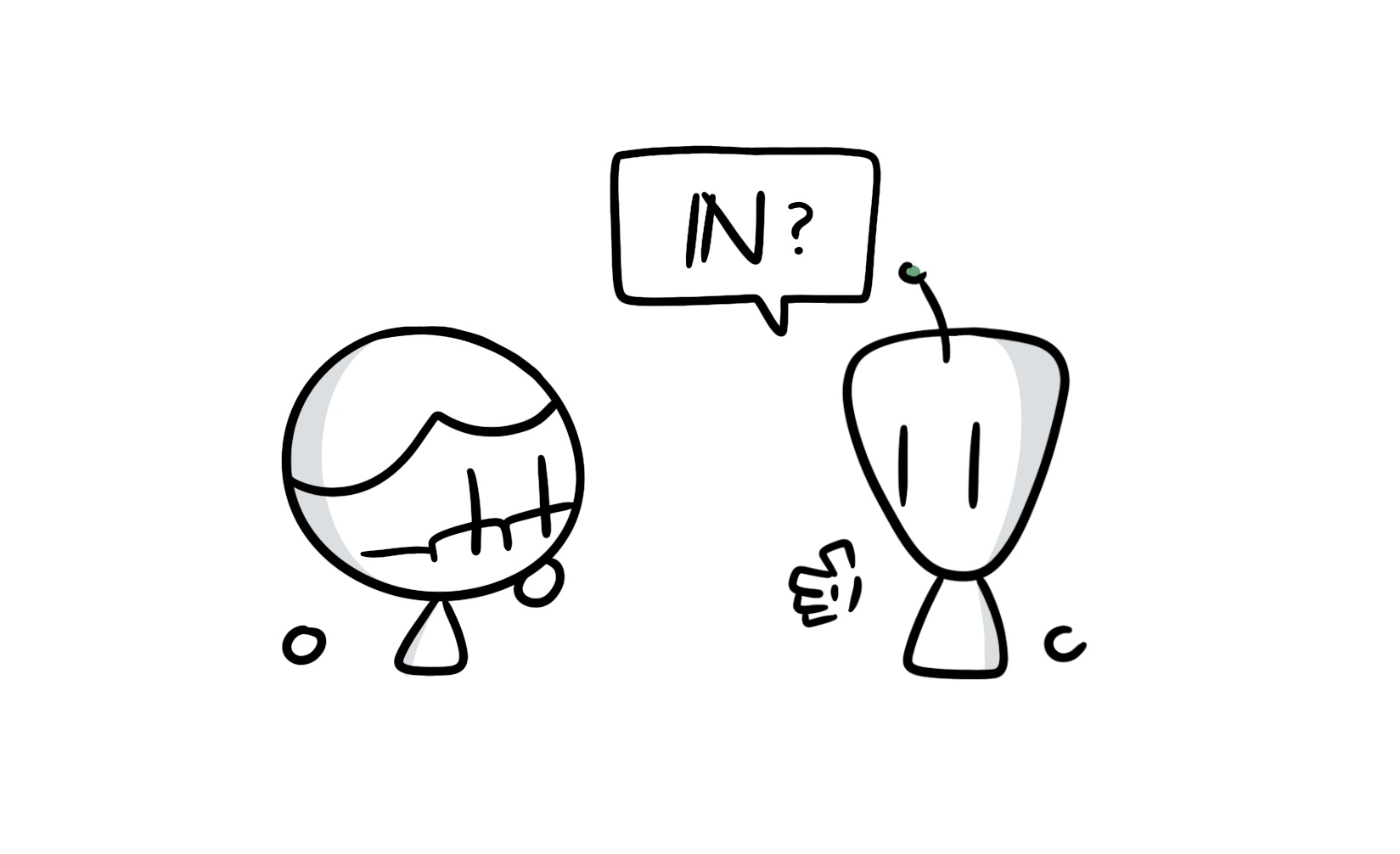
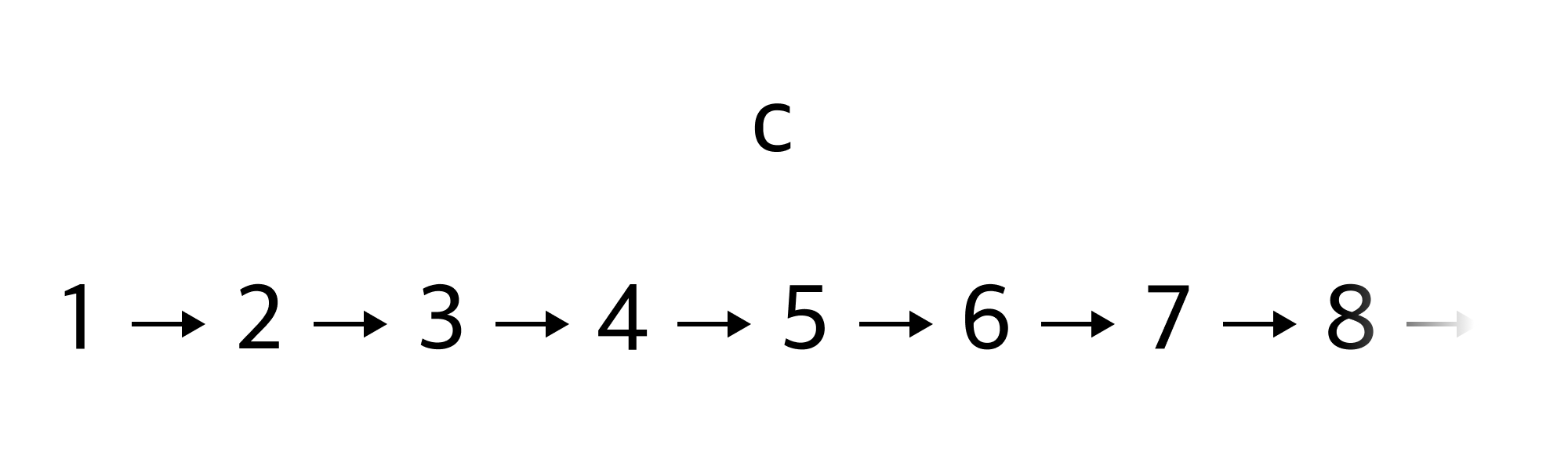
뭐긴 뭐야. 자연수란 1부터 시작해서 2, 3, … 이렇게 순서대로 나아가는 수 체계야.
외계인음…그러면 이것도 자연수야?
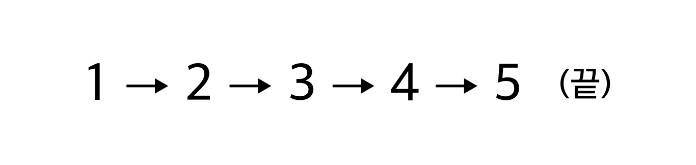
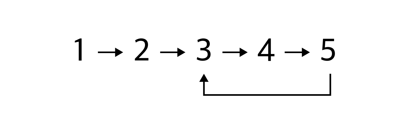
엥, 그럴 리가! 자연수는 끝없이 이어져.
외계인끝없이 이어진다고? 고리를 이룬다는 말인가? 그럼 1, 2, 3, 4, 5, 3, 4, 5, 3, 4, 5, … 이렇게 끝없이 이어지는데.
맙소사, 그 뜻이 아니야. 고리 같은 거 없이 끝없이 이어져.
외계인흠...그럼 중간에 가지라도 치나?
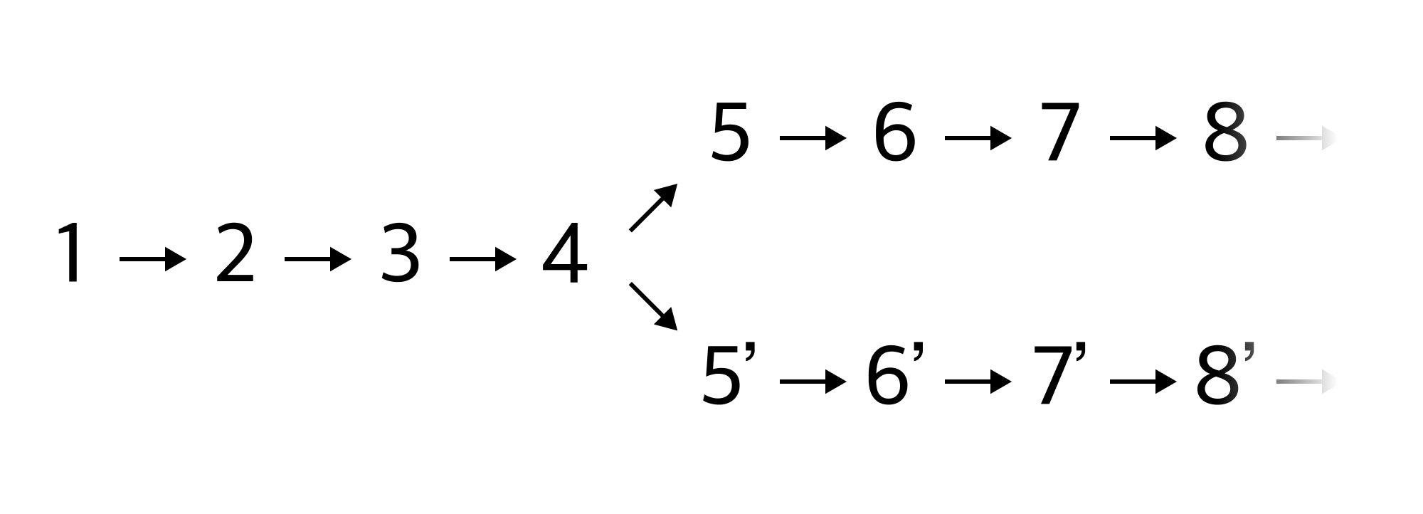
그것도 아니야! 가지는 없어!
외계인알겠어. 그렇다면 혹시 $c$도 자연수니?
디멘$c$라니, 무슨 말이야?
외계인너가 알려준 자연수의 정의대로라면 $c$가 자연수가 아닐 이유는 없는데? 자연수는 끝없이 이어진다고 했지만 모든 자연수가 그러한 연쇄에 포함된다고 말하지는 않았잖아.
저건 또 뭐야... 자연수에는 자연수밖에 없어!
외계인자연수에는 자연수밖에 없다니, 순환논법이 따로 없네.
디멘너 지금 나 놀리는 거지?
외계인무슨 소리야, 난 진짜 자연수가 뭔지 모르겠어. 너야말로 자연수의 정의를 제대로 알려줘야 내가 이해를 할 거 아니야.
디멘자연수란...음...그러니까...하, 이걸 어떻게 설명하지!
그 순간, 데데킨트라는 사람이 나타났습니다.
내가 이 문제를 확실히 해결해 주지. 자연수란 다음 세 가지 조건을 만족하는 집합을 말해. 이 세 가지 조건을 만족하는 집합이 유일하다는 사실은 내가 증명해 놓았으니 더 이상 오해의 여지라고는 없지.
데데킨트의 자연수 정의. 집합 $A$, 원소 $e \in A$, 그리고 함수 $S: A \to A$가 다음 세 가지 조건을 만족한다면 $A, e, S$는 각각 자연수 집합, $0$, 그리고 $x \mapsto x + 1$에 대응된다.
- $S(x) = e$를 만족하는 $x$는 존재하지 않는다.
- $S(x) = S(y)$라면 $x = y$이다.
- $A$를 정의역으로 하는 임의의 명제 $P(x)$에 대해 다음 두 조건이 성립한다면 $P(x)$는 $A$의 모든 원소에 대해 참이다.
- $P(e)$가 참이다.
- $P(x)$가 참이라면 $P(S(x))$가 참이다.
데데킨트의 대답에 외계인은 흡족해했지만, 이내 또다시 의아하다는 표정을 지었습니다.
세 번째 조건에 "임의의 명제"라는 표현이 말이 돼? $P(x)$가 임의의 명제라면 $P(x)$는 "$x$가 자연수이다" 가 될 수도 있잖아. 하지만 자연수의 정의에 자연수에 대한 명제가 포함되는 건 순환논법일 텐데?
데데킨트엇...그런가...?
외계인애초에 "명제"라는 것이 정확히 뭐야? "$x$는 자기 자신을 포함하지 않는 집합이다" 는 잘 정의된 명제야?
디멘(만약 $x$가 자기 자신을 포함하지 않는 집합이라면 $x$는 $x$의 정의에 해당하므로 자기 자신을 포함하게 되고, $x$가 자기 자신을 포함하는 집합이라면 $x$는 $x$의 정의에 해당하지 않으므로 자기 자신을 포함하지 않게 되고...엥?)
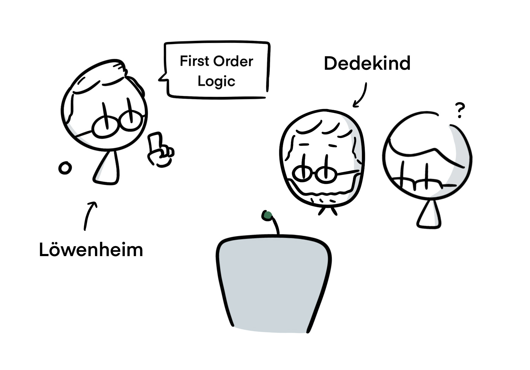
뜻밖의 지적에 데데킨트가 우물쭈물하자 옆에서 뢰벤하임이라는 사람이 끼어들었습니다.
확실히 "임의의 명제"라는 표현은 문제가 있어 보이네. 아무래도 수학에서 이런 표현은 제한해야겠어. 이렇게 제한된 논리학을 1차 논리라고 부르자.
그렇다면 이제 어떻게 1차 논리로 자연수를 정확하게 정의할 수 있는지 알아봐야겠군.
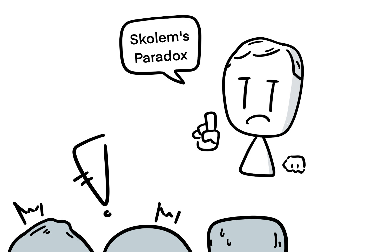
이 말에 스콜렘이라는 사람이 불쑥 나타났습니다.
맞아. 그리고 내가 이 질문에 대한 답을 발견했어.
스콜렘의 발언에 모두가 주의를 집중했습니다.
불가능해. 1차 논리로는 자연수의 필요충분조건을 기술할 수 없어. 구체적으로, 자연수의 정의를 시도하는 모든 1차 논리적 정의에는 자연수가 아닌 반례가 존재해. 따라서 자연수는 논리로 환원될 수 없어. 자연수를 순환논법 없이는 정의할 수 없다는 말이야.
뢰벤하임-스콜렘 정리. 자연수를 비롯하여, 원소가 무한히 많은 수 체계는 1차 논리로 유일하게 특정될 수 없다.
순간 정적이 흘렀습니다.
그렇다면 인간들은 어떻게 자연수가 뭔지 아는 거야? 알고 보면 인간들은 저마다 자연수를 다르게 알고 있는 거 아냐?
외계인의 질문에 아무도 대답하지 못했습니다. 그들은 신기루 같은 자연수의 실체에 대해 할 말이 더 이상 남아 있지 않았습니다.
Note. 이야기의 자연스러운 흐름을 위해 왜곡된 역사적 · 수학적 · 철학적 내용이 있습니다. 1차 논리의 탄생은 뢰벤하임을 비롯한 여러 수학자들의 점진적인 연구로 이루어졌습니다. 또한 데데킨트의 자연수 정의가 사용하는 2차 논리가 정말로 순환적인지에 관해서는 더 자세한 논의가 필요합니다. 마지막으로 스콜렘의 역설은 자연수에 관한 것이 아닌 집합론에 관한 것인데, 뢰벤하임-스콜렘 정리의 귀결이라는 점에서 두 현상은 유사하기 때문에 말풍선에 넣었습니다.
더 읽어보기
Natural Numbers as a Mirage: A Short Story in Logic
14 Sep 2025This post was originally written in Korean, and has been machine translated into English. It may contain minor errors or unnatural expressions. Proofreading will be done in the near future.
One day, Dimen encountered an alien. The alien asked Dimen:
There's a concept that humans use which I don't understand. What exactly are natural numbers?
What do you mean? Natural numbers are a number system that starts from 1 and proceeds sequentially: 2, 3, … and so on.
AlienHmm... Then are these also natural numbers?
No way! Natural numbers continue indefinitely.
AlienContinue indefinitely? Do you mean they form a loop? Then they would continue indefinitely like this: 1, 2, 3, 4, 5, 3, 4, 5, 3, 4, 5, …
Good heavens, that's not what I meant. They continue indefinitely without any loops.
AlienHmm... Then do they branch somewhere?
That's not it either! There are no branches!
AlienI see. Then is $c$ also a natural number by any chance?
Dimen$c$? What do you mean?
AlienAccording to the definition of natural numbers you've given me, there's no reason why $c$ shouldn't be a natural number. You said natural numbers continue indefinitely, but you didn't say that all natural numbers are included in such a chain.
What is that supposed to be... Natural numbers contain only natural numbers!
AlienNatural numbers contain only natural numbers—that's nothing but circular reasoning.
DimenAre you making fun of me?
AlienWhat are you talking about? I genuinely don't understand what natural numbers are. You need to give me a proper definition of natural numbers for me to understand.
DimenNatural numbers are... well... that is... ugh, how do I explain this!
At that moment, a person named Dedekind appeared.
I shall resolve this problem definitively. Natural numbers are a set that satisfies the following three conditions. I have proven that a set satisfying these three conditions is unique, so there is no room for further misunderstanding.
Dedekind’s definition of natural numbers. If a set $A$, an element $e \in A$, and a function $S: A \to A$ satisfy the following three conditions, then $A$, $e$, and $S$ correspond to the set of natural numbers, $0$, and $x \mapsto x + 1$, respectively.
- There exists no $x$ such that $S(x) = e$.
- If $S(x) = S(y)$, then $x = y$.
- For any proposition $P(x)$ with domain $A$, if the following two conditions hold, then $P(x)$ is true for all elements of $A$:
- $P(e)$ is true.
- If $P(x)$ is true, then $P(S(x))$ is true.
The alien was satisfied with Dedekind’s answer, but soon looked puzzled again.
Does the expression "any proposition" in the third condition make sense? If $P(x)$ is any proposition, then $P(x)$ could be "$x$ is a natural number". But including a proposition about natural numbers in the definition of natural numbers would be circular reasoning, wouldn't it?
DedekindOh... is that so...?
AlienWhat exactly is a "proposition" anyway? Is "$x$ is a set that does not contain itself" a well-defined proposition?
Dimen(If $x$ is a set that does not contain itself, then $x$ satisfies the definition of $x$, so it contains itself; but if $x$ is a set that contains itself, then $x$ does not satisfy the definition of $x$, so it does not contain itself... huh?)
As Dedekind hesitated at this unexpected criticism, a person named Löwenheim interjected from the side.
Indeed, the expression "any proposition" seems problematic. We should restrict such expressions in mathematics. Let us call this restricted logic first-order logic.
Then we must now discover how to define natural numbers precisely using first-order logic.
At these words, a person named Skolem suddenly appeared.
Precisely. And I have discovered the answer to this question.
Everyone focused their attention on Skolem’s statement.
It's impossible. First-order logic cannot describe the necessary and sufficient conditions for natural numbers. Specifically, every first-order logical definition that attempts to define natural numbers has counterexamples that are not natural numbers. Therefore, natural numbers cannot be reduced to logic. Natural numbers cannot be defined without circular reasoning.
Löwenheim-Skolem theorem. Mathematical systems with infinitely many elements, including natural numbers, cannot be uniquely characterised by first-order logic.
A moment of silence followed.
Then how do humans know what natural numbers are? Don't humans actually understand natural numbers differently from one another?
No one could answer the alien’s question. They had nothing more to say about the mirage-like reality of natural numbers.
Note. For the natural flow of the narrative, there are distorted historical, mathematical, and philosophical contents. The birth of first-order logic was achieved through the gradual research of several mathematicians, including Löwenheim. Moreover, whether Dedekind’s definition of natural numbers using second-order logic is truly circular requires more detailed discussion. Finally, Skolem’s paradox concerns set theory rather than natural numbers, but it was included in the speech bubble because the two phenomena are similar as consequences of the Löwenheim-Skolem theorem.
Further Reading
자연주의적 목적론은 논리를 설명할 수 있는가?
13 Sep 2025이 글은 제가 작성한 소논문입니다. 원문이 영문으로 작성되었고, 주제 또한 영미철학이기 때문에, 영문 버전이 글 자체는 훨씬 더 자연스럽습니다. (영문 PDF: 링크)
초록
이 글은 원초적 지향성original intentionality에 대한 데넷의 회의주의와, 자연주의적 목적론natural teleology으로 언어의 의미를 해명하고자 하는 데넷의 시도를 두 단계에 걸쳐 검토한다. 첫째, 데넷의 회의주의가 의존하는 불확정성 문제indeterminacy problem는 그 자체로 원초적 지향성을 반박하지 못한다고 논증한다. 둘째, 논리에 대한 자연주의적 목적론 설명은 순환논리에 빠진다고 논증한다. 따라서 논리는 원초적 지향성이 성립해야 하는 영역임을 결론내린다.
1. 서론
1.1. 원초적 지향성 논제The Doctrine of Original Intentionality
데넷(1981)은 마음의 지향성을 둘러싼 논의에서 중대한 견해 차이를 관찰한다. 이 견해 차이는 원초적 지향성에 관한 것으로, 데넷은 이를 다음과 같이 제시한다:
원초적 지향성 논제란, 우리의 인공물 중 일부는 우리로부터 파생된derived 지향성을 가지지만, 우리는 완전히 파생되지 않은 원초적 지향성을 갖는다는 주장이다.
데넷은 다음 예시로 이를 설명한다. 미국 동전을 받아들이는 자판기를 생각해보자. 자판기가 미국 동전을 받아들일 때 기계는 x는 미국 동전이다를 “의미하는” 상태state Q에 들어간다고 하자. 흥미롭게도 자판기는 파나마 동전과 미국 동전을 구별할 수 없다. 그렇다면 자판기가 파나마 동전을 받아들일 때, 기계가 상태 Q에 들어간다고 해야 할까(“잘못된” 표상representation), 아니면 x는 파나마 동전이다를 “의미하는” 새로운 상태 B에 들어간다고 해야 할까(“올바른” 표상)?
직관적인 답은 설계자의 의도intention에 달려 있다는 것이다. 미국인 기술자가 미국 동전을 식별할 의도로 자판기를 설계하여 미국에 설치했다면, 기계는 상태 Q에 들어가며, 파나마 동전이 투입되면 잘못된 표상이 발생한다. 설계자가 파나마인이었다면 그 반대가 될 것이다. 따라서 기계의 지향성은 설계자의 것으로부터 파생된 것이다.
여기까지는 논란의 여지가 없다. 자판기가 단순한 인공물에 불과하기 때문이다. 논쟁은 이 결론이 과연 인간에게도 성립하는지에 관한 것이다. 가령 다음의 경우를 생각해 보자. 일반적으로 존스가 말을 보고 “말”이라고 말할 때, 그는 x는 말이다를 의미하는 상태 H에 있다고 여겨진다. 어느 날 존스가 말과 닮았지만 분류학적으로는 말이 아닌 생물인 슈모스schmorse와 마주친다. 이 사건이 존스에게 일으키는 상태는 상태 H인가, 아니면 x는 슈모스다를 의미하는 새로운 상태 SH인가? 아니면 줄곧 존스에게 해당했던 상태는 H가 아니라 x는 말이거나 슈모스거나 …를 의미하는 상태 H*였던 것인가?
여기서 데넷은 전선을 그어놓는다:
그가 정확히 어떤 상태에 있는지 결정하기가 아무리 어렵더라도 그는 실제로 둘 중 하나의 상태에 있다… 이 직관을 거부할 수 없다고 생각하는 사람은 원초적 지향성을 믿는 것이며, 훌륭한 동료들이 있다: 포더, 설, 드레츠케, 버지, 크립키… 이 직관을 의심스럽다고 생각하거나 완전히 기각 가능하다고 여기는 사람은 나, 처칠랜드 부부, 데이비슨, 하우겔란드, 밀리컨, 로티, 스탈네이커, 그리고 우리의 뛰어난 선배들인 콰인과 셀라스와 함께 다른 편에 설 수 있다.
1.2. 데넷의 대자연Mother Nature
데넷은 개인에 관한 어떤 사실로도 그의 정신 상태에 관한 불확정성 문제를 해결할 수 없다고 주장한다. 불확정성을 해결하는 데 필요한 것은 우리의 지향성이 자판기의 것만큼 파생된 것임을 인식하는 것이다. 다만 설계자가 인간이 아니라 자연사라는 점이 다를 뿐이다.
예를 들어, 개구리가 납 구슬을 파리로 착각하여 “잘못” 낚아챈다는 것은 잘 알려진 사실이다. 그런데 왜 그것이 오류일까? 만약 개구리의 낚아침과 결부된 상태의 의미가 “파리를 낚아챔”이었다면, 납 구슬을 낚아채는 것은 분명 오류이다. 그러나 결부된 상태의 의미가 “파리 또는 납 구슬을 낚아챔”이었다면 오류가 아니다. 무슨 근거로 우리는 개구리의 낚아침에 결부된 의미가 후자가 아닌 전자라고 주장할 수 있는 것일까?
데넷의 요지는, 그 근거를 개구리의 신경생리학이 아닌, 개구리로 하여금 특정 대상들을 낚아채게 만든 자연선택의 역사에서 찾아야 한다는 것이다. 자연선택의 논리에서 보았을 때 개구리의 낚아채기는 영양분을 얻는 목적을 “위해 선택되었음selected for“이 분명해지므로, 개구리가 납 구슬을 낚아채는 것은 실수다. 따라서 자판기와 마찬가지로 개구리의 지향성은 설계자로부터 파생된 것이다. 차이점은, 설계자가 “대자연”이라는 것이다. 나아가 데넷은 개구리의 지향성이 파생적이라면, 인간 또한 개구리와 동일한 원리에 의해 진화했으므로 우리의 지향성 또한 파생적이라고 결론내린다.
포더(1996)를 따라, 데넷의 입장을 세 부분으로 더 정확히 “해체”할 수 있다: (1) 적응주의adaptationism가 자연선택의 참된 설명이다. (2) 적응주의는 자연주의적 목적론natural teleology—자연이 어떤 목적을 “위해” 특정 기관 또는 기능을 “선택한다”고 말하는 방식—을 정당화한다 (자연주의적 목적론의 명제들은 진릿값을 가진다). (3) 자연주의적 목적론은 지향성과 의미를 정초한다.
이 글에서는 (1)과 (2)를 단순히 받아들이는 것으로 시작할 것이다. 예컨대 혈액을 순환시키는 심장들의 집합과, 맥박 소리를 내는 심장들의 집합이 외연적으로 일치한다는 것은 아마 법칙적 필연nomologically necessity이지만, “심장은 맥박 소리를 내는 능력을 위해 선택되었다”는 거짓이고 “심장은 혈액을 순환시키는 능력을 위해 선택되었다”는 참임을 인정할 것이다. 이 글의 논지는, 그럼에도 불구하고 자연주의적 목적론은 특정 부류의 지향성을 설명하기에 충분하지 않다는 것이다.
2. 문제의 재구성
2.1. 불확정성 문제는 “공정”한가?
데넷이 불확정성 문제를 원초적 지향성을 의심하는 주요 이유로 인용하므로, 문제의 정확한 구조를 다음과 같이 명료화하는 것이 논의에 도움이 될 것이다.
- 지향적 실재론자들intentional realists(원초적 지향성의 지지자들)은 다음을 주장한다:
- 표상적 정신 상태representative mental state라 불리는 정신 상태의 부류가 있다.
- 각각의 표상적 정신 상태는 세계가 특정한 방식으로 존재한다고 표상하는 내용content을 갖는다.
- 행위자가 표상적 정신 상태에 있다면, 그가 어떠한 정신 상태에 있는지에 관해 불확정성이 있어서는 안 된다.
- (1.2)로부터 다음이 따른다:
- 표상적 정신 상태가 주어지면, 그것이 세계를 올바르게 표상하는지에 관해 불확정성이 있어서는 안 된다.
- (1.3)과 (2.1)로부터 지향적 실재론자들이 다음을 주장한다는 것이 따른다:
- 행위자가 표상적 정신 상태에 있다면, 그의 상태가 세계를 올바르게 표상하는지에 관해 불확정성이 있어서는 안 된다.
- 따라서 (3.1)에 대한 반례가 있다면, 지향적 실재론은 거짓이다.
데넷은 앞서 언급한 말-슈모스 사례뿐만 아니라 퍼트남의 H₂O-XYZ 사례, 그리고 자신의 glug 사례(데넷 1981)를 포함하여 (3.1)에 대한 다양한 반례를 인용한다. 그러나 나는 위에서 서술된 형태의 불확정성 문제는 잘못 설정되었다고 주장한다. 왜냐하면 설령 지향적 실재론이 참이더라도, (3.1)에 대한 반례는 항상 존재하기 때문이다.
가령 (1.1), (1.2), (1.3)을 인정하고, 존스가 “의자”라고 말할 때 그는 x는 의자다라는 내용을 가진 표상적 정신 상태에 있다고 하자. 이제, $s_1$은 의자이고 $s_n$은 톱밥 더미인 소라이츠 열Sorites sequence $(s_1, \dots, s_n)$을 고려해보자. (3.1)은 존스가 “의자”라고 말할 때 $1 ≤ i ≤ n$에 대해 $s_i$를 올바르게 표상하는지에 관한 기준이 있어야 한다고 요구한다. 그러나 그런 기준은 없으므로 (3.1)은 반박된다.
그러나 이것은 지향적 실재론에 대한 유효한 반박이 될 수 없다. 기껏해야 “의자”와 연관된 내용의 모호성vagueness을 드러낼 뿐이다. 불확정성 문제의 오류는 (1.2)로부터 (2.1)을 연역하는 데 있다1. 즉, 표상은 어떤 세계들이 올바른지에 대한 미리 결정된 기준 없이도, 세계가 특정한 방식으로 존재한다고 표상할 수 있다. 가령, 소라이츠 열 중 어디부터가 의자에 해당하는지에 관한 명백한 기준이 없더라도 의자라는 개념은 표상될 수 있다. 여기서의 교훈은 의미가 불확정적이라는 것이 아니라, 확정적인 의미가 모호한 외연을 가질 수 있다는 것이다.2
그렇긴 하지만, 이 지적이 데넷의 예시들에 어느 정도 유효한지는 명확하지 않다. 반쯤 부서진 의자들에 대해 “의자”라고 말하는 것의 모호성이 슈모스들에 대해 “말”이라고 하는 것과 동일시될 수 있을까? 생물학적 종에 대한 반실재론자들은 그렇게 보려 할 것이지만, 본질주의자들은 둘을 같은 선상에 놓는 것이 절박한 시도라고 반박할 것이다.3
이 문제를 계속 논의할 수도 있지만, 이는 의도치 않은 형이상학적 굴레로 빠지는 일이다. 따라서 나의 제안은 데넷의 불확정성 예시들이 실제로 지향적 실재론을 위협하는지의 문제를 제쳐두는 것이다. 구체적으로 말하자면, 의자나 말 등의 물리적 대상을 통해 불확정성 문제를 제기하는 방식을 배제하고, 대신 만약 의미가 존재한다면 결코 그 의미가 모호할 수 없는 언어 및 대상들에 한해 불확정성 문제를 논의하는 것이 더 나은 진행 방식이라고 생각한다. 이는 우리로 하여금 논리로 초점을 이동하게 한다.
2.2. 논리와 수학에서의 불확정성
크립키(1982)의 유명한 회의적 역설은 50보다 높은 수를 더해본 적이 없는 화자가 ‘+’로 덧셈을 의미했는지, 아니면 컷셈quaddition(아래에 정의됨)을 의미했는지에 관한 사실이 있는지 묻는다.
\[x \oplus y = \begin{cases}x + y & (x, y < 50) \\5 & \text{(otherwise)}\end{cases}\]곧 드러날 이유 때문에, 나는 크립키의 사례를 약간 변형하여 산술 대신 논리에 적용할 것이다. 가령 함의 기호 ‘→’를 고려해보자.4 캄의quimplication를 50개 미만의 토큰을 가진 문장 안에서는 함의와 일치하고, 그렇지 않은 문장은 언제나 거짓으로 만드는 연산이라고 하자. 예를 들어, $p \to p$는 참이지만, $(p_1 \land p_2 \land \dots \land p_{50}) \to p_1$은 거짓이다.
앨리스가 평생에 걸쳐 50개보다 많은 토큰을 가진 문장을 단 한 번만 다루었다고 가정하자(더 극적인 시나리오를 위해 그녀가 죽어서 그녀의 언어 사용에 관한 추가 데이터를 얻을 수 없다고 생각해도 좋다). 해당 문장 φ는 참이었지만 앨리스는 φ를 거짓으로 판단했다. 그런데 만약 ‘→’가 캄의를 의미했다면 그 문장은 실제로 거짓이었다고 가정하자. 이제 우리는 말-슈모스 사례와 유사한 불확정성에 직면한다. 앨리스는 ‘→’로 함의를 의미했지만 오류를 범한 것일까, 아니면 앨리스는 ‘→’로 캄의를 의미했고 정확한 사용을 한 것일까?
나는 ‘→’의 불확정성 문제가 여타 불확정성 문제보다 지향성을 논의하기에 더 적합하다고 주장한다. 이제 불확정성을 내용의 모호성 탓으로 돌릴 수 없기 때문이다.5 그러므로 지향성의 불확정성 문제를 다음과 같이 재구성하자. 우리가 “함의한다”와 같은 논리적 어휘를 사용할 때, 우리는 확정적인 의미를 가진 정신 상태에 있는가? 이제 데넷주의자가 이 질문에 어떻게 응답할지 개괄하고, 그런 응답들이 순환논리에 빠진다고 논증할 것이다. 따라서 원초적 지향성 논제는 적어도 우리의 논리 사용에 대해서는 참이어야 한다.
3. 논리에 대한 논증
3.1. 논리에 대한 데넷주의적 관점
추정컨대 데넷주의자는 “앨리스가 ‘→’로 함의를 의미한다”와 “앨리스가 ‘→’로 캄의를 의미한다”는 진술 모두가 정당화된다고 주장할 것이다. 실제로 두 진술은 모두 데넷(1991)에서 제시된 “실재 패턴real patterns“의 기준을 만족한다. 둘 다 앨리스의 ‘→’ 사용을 그녀의 행동에서의 패턴, 즉 “앨리스가 ‘A’와 ‘A → B’를 승인할 때, 그녀는 ‘B’를 승인하는 성향이 있다”와 같은 진술로써 구성된다. 차이점은, 후자의 경우 ‘A → B’의 토큰 수가 50개 미만이어야 한다는 조건이 추가된다는 것이다. 이 차이에도 불구하고 두 패턴은 모두 실재적이다. 즉, 존스가 첫 번째 패턴을, 브라운이 두 번째 패턴을 사용하여 앨리스의 미래 ‘→’ 사용을 예측하고 그에 따라 내기를 했다면, “둘 다 부자가 될 것”이라는 의미에서 실재적이다.
그러나 더 야심찬 데넷주의자는 불확정성에 그렇게 쉽게 굴복하지 않을 수도 있다. 대신 자연주의적 목적론을 통해 ‘캄의’보다 ‘함의’ 해석을 정당화하려고 시도할 수 있다. 앞서 자연주의적 목적론이 개구리가 납 구슬을 낚아채는 것을 실수라고 말할 수 있는 길을 열어주는 것을 보았다. 개구리의 물건을 낚아채는 능력이 영양분을 얻는 기능을 위해 “선택되었기selected for” 때문이다. 데넷주의자는 논리에 대해서도 마찬가지로 논증할 수 있다. 논리로 추론하는 우리의 능력은 참인 전제들로부터 참인 문장들을 연역하는 기능을 위해 “선택되었는데”, 이는 거짓보다 참을 더 많이 아는 것이 진화적으로 유리하기 때문이다. 그런데 ‘→’를 캄의로 해석하는 연역은 모순적이므로, 앨리스는 ‘→’로 함의를 의미했으며, φ를 참이라고 판단한 것은 오류였다는 결론이 따른다.
3.2. 논리, 참, 그리고 효용
그러나 나는 이런 시도가 참truth 개념에 호소한다는 점에서 문제가 있다고 주장한다. 타르스키 이후로 잘 알려진 사실은 참의 개념이 언어에 상대적이라는 것이다. 따라서 데넷주의자가 “앨리스가 참인 문장들을 많이 알수록 앨리스에게 진화적으로 유리하다”라고 주장할 때, 여기서 “참”은 실제로 “$L_A$에서-참”을 의미한다 ($L_A$는 앨리스의 언어를 나타낸다).
중요하게도, 솜즈(1984)는 언어의 범위가 논리적 어휘를 포함한다고 지적한다. 따라서 다음과 같은 타르스키적 참 정의의 조항들은, ($T_A$는 “$L_A$에서-참”을 나타낸다)
(1) $T_A(\ulcorner \phi \;\dot{\to}\; \psi \urcorner)$ iff $T_A(\ulcorner \phi \urcorner)$가 $T_A(\ulcorner \psi \urcorner)$를 함의한다 6
‘→’가 앨리스의 언어에서 함의를 의미한다는 사실을 전제한다. 이 전제 없이는 참의 정의가 시작조차 될 수 없다. 솜즈는 이 점을 사용하여 필드(1972)가 구상한 참의 물리주의적 환원에 대해 논증하지만, 우리는 그의 점을 사용하여 논리에 대한 자연-목적론적 설명에 대한 공격을 전개할 수도 있다. 자연-목적론적 설명은 참, 구체적으로 “$L_A$에서-참”의 효용에 호소하여 앨리스가 사용하는 논리적 어휘의 (파생된) 의미들이 무엇인지 결정한다. 그러나 “$L_A$에서-참”의 바로 그 정의가 해당 의미에 의존하므로, 순환논리에 빠진다.
그러나 데넷주의자들은 어떠한 참 개념에 호소해야만 한다. 특정 부류의 문장들과 연역들이 다른 것들보다 더 “진화적으로 유리”할 수 있는 이유로서, 참의 효용utility of truth 말고는 후보가 없기 때문이다.7 데넷주의자들이 취할 수 있는 다른 한 가지 방법은 “$L_A$에서-참”을 앨리스가 믿었을 때 그녀에게 유용할 문장들의 부류로 단순히 정의하는 것이다. 이는 실용주의적 진리론을 채택하는 것이고, 참이 진화적으로 유익하다는 주장은 자명하게 따라올 것이다. 그러나 이 경우에는 함의가 캄의보다 더 진리-보존적(즉 효용-보존적)인 이유가 불분명할 뿐만 아니라, 함의가 실제로 캄의보다 더 진리-보존적(효용-보존적)인지조차 불분명하다 (물론 실용주의 이론을 학계에서 사장되게 만든 더 심각한 문제들도 있다).
그렇다면 데넷주의자들은 수축주의deflationism를 채택함으로써 참에 대한 실질적 설명을 제공하는 것을 단순히 우회하는 선택을 할 수 있을까? 관건은 수축주의가 참의 효용을 설명할 수 있는지이다. 버지스(2011)는 그러한 설명의 개략을 제시한다. 어떤 믿음이, 해당 믿음을 갖는 것이 의지력이 약하지 않은not weak-willed 한 행위자로 하여금 특정한 행동을 하게 한다면, 그 믿음을 직접적으로 행동-안내적directly action-guiding이라고 하자. 예를 들어 다음의 믿음은 직접적으로 행동-안내적이다.
(2) 지금 헬스장에 가는 것은 가장 선호하는 결과로 이어질 것이다.
믿음이 행위자의 가장 선호하는 결과를 얻는 데 유용한 경우 해당 믿음을 유용하다고 하자. (2)가 유용한 믿음일 필요충분조건은 지금 헬스장에 가는 것이 화자에게 가장 선호되는 결과로 이어질 것이다. 그런데 이는 수축주의적 진리관에서 (2)가 참이라고 말하는 것과 동치다. 즉, (2)가 유용할 믿음일 필요충분조건은 (2)가 참인 것이다. 따라서 수축주의자들은 적어도 직접적으로 행동-안내적인 믿음들에 대해서는 참의 효용을 설명할 수 있다.
버지스는 이 접근법을 일반적인 경우로 확장한다. 핵심 아이디어는, “직접적으로 행동-안내적인 믿음들은 보통 다른 믿음들을 전제로 삼아 추론된 결론들일 것이므로, 전제가 된 믿음들이 참이고, 전제로부터 결론을 추론하는 방식이 진리-보존적이라면, 해당 전제들은 간접적으로 유용하다”는 것이다. 구체적인 예시를 들어보자. 만약 다음 두 명제에 대한 앨리스의 믿음이,
(3) 만약 내가 오늘 급한 마감일이 없다면, 지금 헬스장에 가는 것은 가장 선호하는 결과로 이어질 것이다.
(4) 나는 오늘 급한 마감일이 없다.
앨리스로 하여금 (2)를 믿게 만든다면, 다음이 따른다:
- (2)가 유용한 믿음이라면, (3)과 (4)는 간접적으로 유용한 믿음들이다.
- 지금 헬스장에 가는 것이 앨리스에게 가장 선호하는 결과로 이어진다면, (2)는 유용한 믿음이다.
- (a) 만약 앨리스가 오늘 급한 마감일이 없다면 지금 헬스장에 가는 것은 가장 선호하는 결과로 이어질 것이고, (b) 앨리스가 오늘 급한 마감일이 없다면, 지금 헬스장에 가는 것이 앨리스에게 가장 선호하는 결과로 이어진다.
- (a)는 (3)이 앨리스에게 참이라고 말하는 것과 같고 (b)는 (4)가 앨리스에게 참이라고 말하는 것과 같다.
- 따라서 (3)과 (4)가 앨리스에게 참이라면 (3)과 (4)는 간접적으로 유용한 믿음들이다.
이 설명이 수축주의자에게는 만족스러울 수 있지만, 데넷주의자들에게는 문제를 제기한다. 이 설명은 또다시 타르스키적 참 정의에 암묵적으로 의존하기 때문이다. 즉, (3)이 앨리스에게 참이라는 것이 (a)와 같다고 말할 수 있기 위해서는 앨리스가 “…라면”으로 함의를 의미한다는 사실이 전제되어 있다. 만약 앨리스가 “…라면”으로 함의가 아닌 캄의를 의미했다면, (3)의 참 (구체적으로, (3)의 “$L_A$에서-참”) 은 (a)가 아니라 (c)와 같다.
(c) 캄약 앨리스가 오늘 급한 마감일이 없다면, 지금 헬스장에 가는 것은 가장 선호하는 결과로 이어질 것이다.
그러나 (c)와 (b)는 지금 헬스장에 가는 것이 앨르시에게 가장 선호되는 결과로 이어질 것이라는 사실을 함의하지 않는다.
결론적으로, 참의 효용에 호소하여 행위자가 논리적 어휘로 무엇을 의미하는지 결정하는 모든 자연-목적론적 이야기는 타르스키적 기초를 통해 해당 의미들에 관한 사전 사실들을 전제하므로 순환논리에 빠진다. 따라서 데넷주의자들이 자연주의적 목적론에 호소하여 지향성과 정확성의 어떤 개념을 설명할 수 있다고 하더라도, 논리는 그 중 하나가 될 수 없다.
3.3. 논리의 불확정성은 용인될 수 있는가?
데넷주의자들에게 남은 선택은 앨리스의 논리적 어휘 해석에서의 불확정성을 그 완전한 의미에서 받아들이는 것이다. 이는 다른 모든 사람에게도 동등하게 적용될 것이므로, 논리 일반은 절대적이지도 규범적이지도 않고, 단지 인간들이 일반적으로 따르는 경향이 있는 사고에서의 패턴들에 관한 기술들의 한 집합일 뿐이라는 결론이 따른다.
그러나 19-20세기 독일어권 세계에서 두드러지게 특징지어진 잘 발달된 사고의 흐름은 논리에 대한 그러한 관점이 비정합적이라고 주장한다. 이 흐름은 당시 유행했던 심리주의에 대한 반작용으로 발전되었다. 심리주의는 심리학이 사람들이 그렇게 생각하는 이유를 설명하는 경험과학이고, 논리가 사고의 규칙성에 관한 것이므로, 논리가 심리학에 포섭된다고 주장한다.
데넷의 관점을 “심리학”을 신경생리학과 행동주의를 포함하도록 해석한 심리주의와 동일시하고 싶은 유혹이 있지만, 이런 비난 자체는 부당할 것이다. 데넷이 어떤 의미에서의 규범성을 확보할 수 있었을 자연주의적 목적론 접근을 구비하고 있기 때문이다. 그러나 이제 이 접근이 논리에 대해서는 효과적이지 않다는 것을 보았으므로, 데넷주의적 관점은 실제로 완전한 심리주의에 연루되어 있고, 심리주의에 대해 제기된 어려움들에 취약한 것으로 보인다.
그러나 이런 어려움들을 조사하는 대신, 심리주의의 어려움들이 어떻게든 극복될 수 있다고 하더라도, 그것이 데넷주의적 관점과 관련하여 일관성이 있을 수 없다는 추가적인 이유들이 있다고 지적하는 것이 이 글에서는 더 적절할 것이다. 데넷주의적 관점에 독특한 것은 정신적 내용들에 대한 제거주의와 실재론 사이의 중간 입장을 유지하려고 시도한다는 것이기 때문이다. 데넷은 민간심리학의 힘을 인정하고 의미나 믿음의 귀속이 정당화된다고 주장함으로써 제거주의와 거리를 두는 한편, 한 사람이 참으로 의미하거나 믿는 것이 무엇인지에 관한 실재적 답이 없다고 주장함으로써 실재론과도 거리를 둔다. 따라서 그는 “한 개인에 대한 두 [불일치하는] 믿음 귀속 체계가 있을 수 있다… 그러나 하나가 그 개인의 실제 믿음들에 대한 기술이고 다른 하나는 그렇지 않다는 것을 확립할 수 있는 더 깊은 사실은 없다”(데넷 1991)와 같은 주장들을 하게 된다.
프레게(1884)는 불일치라는 개념이 공통된 논리적 틀에 대해서만 의미를 갖는다는 점을 유명하게 제기한다. 프레게의 지적이 어떻게 관련되는지 설명하기 위해, 존스와 브라운이 앨리스에게 논리에 관한 두 가지 다른 믿음 체계를 귀속시키는 시나리오를 고려해보자. 존스는 “‘p’와 ‘p → q’로부터 ‘q’를 연역해야 한다”와 같은 표준적인 믿음들을 귀속시키는 반면, 브라운은 앨리스의 행동을 똑같이 잘 설명하는 비표준적 믿음들을 귀속시킨다. 프레게는 다음과 같이 물을 것이다: 브라운과 존스가 귀속시키는 체계들이 진정으로 다르다는 것이 어떻게 입증될 수 있는가? 어쩌면 브라운과 존스가 “$L_A$에서-참”을 다음과 같이 적어 보일지 모른다.
- 존스 주장: “$T_A(\ulcorner \phi \;\dot{\to}\; \psi \urcorner)$ iff $T_A(\ulcorner \phi \urcorner)$가 $T_A(\ulcorner \psi \urcorner)$를 함의한다”
- 브라운 주장: “$T_A(\ulcorner \phi \;\dot{\to}\; \psi \urcorner)$ iff $T_A(\ulcorner \phi \urcorner)$가 $T_A(\ulcorner \psi \urcorner)$를 함의하고, 눈이 희다”
그러나 이것은 그들의 귀속이 다르다는 것을 결정적으로 보여주지 못한다. 존스가 “함의”로 팜의를 의미하여, 두 귀속을 동치로 만들 수 있기 때문이다. 즉, 존스의 언어 $L_J$에서 “$L_J$에서-참”를 $T_J$라고 쓰면, 다음과 같을 수 있다:
- $T_J(\ulcorner \phi \;\dot{\to}\; \psi \urcorner)$ iff $T_J(\ulcorner \phi \urcorner)$가 $T_J(\ulcorner \psi \urcorner)$를 함의하고, 눈이 희다.
이런 무한소급을 피하려면, 공통의 논리적 틀이 확고히 자리잡고 있어야 한다. 브라운과 존스가 둘 다 “함의한다”로 함의를 의미한다는 것이 단순히 주어져야만 우리가 그들이 앨리스에게 논리에 관한 서로 다른 믿음 체계들을 귀속시킨다고 정당하게 말할 수 있다. 그러나 이것은 이 논의를 촉발시킨 회의주의, 즉 원초적 지향성 논제에 대한 회의주의를 반박한다.
결론적으로, 데넷주의적 관점은 논리에 적용될 때 딜레마에 직면한다. 자연-목적론적 설명은 참의 효용에 호소하기 때문에 문제적이다. 그렇다고 단순히 불확정성을 받아들일 수도 없다. 그렇게 하면 우리가 논리적 어휘로 의미하는 것이 확고히 자리잡고 있다고 주어지지 않는 한, 서로 다른 믿음 귀속들이 있다는 것이 불가해하기 때문이다. 어느 경우든 강요되는 결론은 우리의 정신 상태들이 논리적 어휘에 대해 확정적인 의미를 갖는다는 것이다.
4. 결론
다윈의 위험한 아이디어(1994)에서 데넷은 지향성이 “갈고리skyhook“—즉, 원초적 지향성 논제—에 의존하지 않고 “기중기crane“—자연적 목적론—에 의해 완전히 설명될 수 있다는 것을 보이려는 자신의 기획을 설명한다. 그러나 나는 이 그림이 크레인들이 애초에 설 수 있게 하는 바로 그 “기반”을 간과한다고 논증했다. 그 기반은 논리다.
독자들은 이것이 논리와 관련하여 우리를 어떤 입장에 위치시키는지 궁금해할 수 있다. 더 강한 이론이 궁극적으로 우리의 가장 기본적인 지향성을 설명해낸다면 어떨까? 그 질문을 추구하는 것은 이 글의 범위를 벗어난다. 나의 목표는 더 겸손했다: 논리에 대한 자연-목적론적 설명들의 문제점들을 보여주는 것이었다. 지금으로서는 단순히 내가 칸트, 프레게, 비트겐슈타인, 퍼트남에서 발견되는 사고의 흐름—즉, 논리는 설명이 필요한 것이 아니라 모든 설명 행위에서 전제되는 것이라는 사고(퍼트남 2000; 코난트 1992도 참조)—에 호의적이라는 입장을 밝히며 글을 마친다.
참고문헌
- Burgess, Alexis G. & Burgess, John P. (2011). Truth. Princeton University Press.
- Conant, James (1992). The Search for Logically Alien Thought. Philosophical Topics 20 (1):115-180.
- Dennett, Daniel C. (1981). Evolution, error and intentionality. In Daniel Clement Dennett, The Intentional Stance. MIT Press.
- Dennett, Daniel C. (1991). Real patterns. Journal of Philosophy 88 (1):27-51.
- Dennett, Daniel C. (1994). Darwin’s Dangerous Idea. Behavior and Philosophy 24 (2):169-174.
- Ellis, B. (2001). Scientific Essentialism, Cambridge Studies in Philosophy. Cambridge: Cambridge University Press.
- Field, Hartry (1972). Tarski’s Theory of Truth. Journal of Philosophy 69 (13):347.
- Fodor, Jerry (1996). Deconstructing Dennett’s Darwin. Mind and Language 11 (3):246-262.
- Frege, Gottlob (1884/1950). The foundations of arithmetic. Evanston, Ill.,: Northwestern University Press.
- Kripke, Saul A. (1982). Wittgenstein on rules and private language: an elementary exposition. Cambridge: Harvard University Press.
- Kusch, Martin, “Psychologism”, The Stanford Encyclopedia of Philosophy (Spring 2024 Edition), Edward N. Zalta & Uri Nodelman (eds.)
- Putnam, Hilary. (2000). Rethinking mathematical necessity. In A. Crary & R. Read (eds.), The New Wittgenstein, Routledge, pp. 233–249.
- Soames, Scott (1984). What is a theory of truth? Journal of Philosophy 81 (8):411-429.
-
(1.3)이 문제가 될 수 없다는 것, 즉 정신 상태에 내용을 귀속시키는 데 불확정성이 있을 수 없다는 것(정신 상태가 존재한다고 인정하고)은 선험적 참인 것으로 보인다. 내용이야말로 정신 상태의 본질적 속성이고, 따라서 정신 상태를 엄격하게 지시하는 기초가 되어야 하기 때문이다. ↩
-
문제를 더 일반적으로 표현하면, 일부 학자는 자연종natural kinds이 범주적으로 구별된다고 주장한다. 한 종에서 다른 종으로의 부드러운 전이는 있을 수 없다(엘리스 2001). 이 가정 하에서 자연종에 제한된 불확정성 문제들은 (1.1)로부터 (2.1)를 연역하는 것을 허용할 수 있다. 그러나 (1.1)로부터 (2.1)를 추론하는 데 필요한 전제가 존스의 정신 상태에 대한 내용이 모호한 후보가 없다는 것이므로 여전히 어려움이 남아 있다고 생각한다. 이는 존스의 정신 상태에 대한 일부 후보들이 자연종에 해당한다는 진술보다 훨씬 강하다. ↩
-
도움이 된다면 그러한 의미를 초평가주의적supervaluationistic 진리값을 허용하는 결정 트리decision tree로 생각해도 좋다. 의미(결정 트리)는 매우 확정적이다. 단지 그 노드들 중 일부에서 불분명한 값들을 갖는 것뿐이다. ↩
-
편의상 형식논리의 기호들을 설명에 사용하고 있지만, 기호들은 자연언어를 포함하도록 넓게 해석되어야 한다. 따라서 ‘→’는 ‘함의한다’와 ‘만약’도 나타내고, $p \to q$는 “만약 p이면 q다”라는 영어 문장도 나타낸다. 이런 이유로 “논리적 기호들” 대신 “논리적 어휘”라는 표현을 사용할 것이다. ↩
-
이 점은 크립키도 강조한다: “요점은… 내 머릿속의 어떤 것도 ‘plus’(내가 사용하는)가 지시하는 함수가 무엇인지 미결정된 상태로 남겨둔다는 것이다… 회의적 문제는 덧셈 개념의 모호성을 (녹색 개념에 모호성이 있는 방식으로) 나타내지 않는다… 회의적 요점은 다른 것이다.” ↩
-
방점은 대상언어를 메타언어와 구별하는 역할을 한다. 따라서 여기서 $\dot{\to}$는 앨리스가 사용하는 ‘만약’을 나타낸다. ↩
-
데넷(1991)도 이 점을 지적하며 다음과 같이 쓴다: “대응론적 진리론의 무용성을… 본 사람도 자연주의적 존재론적 태도 내에서 우리가 때때로 대응에 의해 성공을 설명한다는 사실을 받아들여야 한다: 메인Maine 해안에서 항해할 때 캔자스Kansas 도로 지도를 사용할 때보다 최신 해도를 사용할 때 더 성공적이다. 왜인가? 전자는 메인 해안의 위험요소, 수심, 해안선을 정확하게 표현하고 후자는 그렇지 않기 때문이다.” ↩
Can Natural Teleology Ground Logic?
13 Sep 2025PDF version: Link
Abstract
This essay examines Dennett’s skepticism about original intentionality and his attempt to ground meaning in natural selection and natural teleology. I argue, first, that the indeterminacy problem on which Dennett’s skepticism relies does not in itself undermine original intentionality; and second, that the natural-teleological account of logic is question-begging due to its appeal to the utility of truth. I conclude that our use of logic demonstrates a domain in which the doctrine of original intentionality must be presupposed.
1. Introduction
1.1. The Doctrine of Original Intentionality
In his 1981 essay, Dennett observes a major disagreement in discussions surrounding the intentionality of the mind. The disagreement is about the doctrine of original intentionality. Dennett puts it as follows:
The doctrine of original intentionality is the claim that whereas some of our artifacts may have intentionality derived from us, we have original (or intrinsic) intentionality, utterly underived.
Dennett illustrates it with the following example. Consider a vending machine, call it “two-bitser”, that accepts U.S. quarters. Allowing ourselves some metaphorical use of language, say that when a two-bitser accepts a quarter, the machine goes into a state Q which “means” x is a quarter. Interestingly, vending machines cannot tell Panamanian balboas and U.S. quarters apart. When a two-bitser accepts a balboa, then, should we say that the machine goes into state Q (hence a “misrepresentation”), or does it go into a new state B which “means” x is a balboa (hence a “correct representation”)?
A straightforward answer is that it depends on the intention of the designer. If an American mechanic designed the two-bitser with the intention of detecting U.S. quarters and installed it in the U.S., the machine goes into state Q, and a balboa fed to the machine triggers a misrepresentation. Had the designer been Panamanian, the opposite would have been the case. Hence the machine’s intentionality is derived from that of the designer.
This much is uncontroversial, since a two-bitser is just an artifact. The debate concerns whether the same is true of humans. It is held prima facie that when Jones sees a horse and utters “horse”, he is in a state H, meaning x is a horse. One day, Jones is confronted with a schmorse, a creature that resembles a horse yet is taxonomically not a horse. Does this encounter cause Jones to be in state H, or does it cause Jones to be in a new state SH meaning x is a schmorse? Or could it have been that it was not state H, but rather state H*, meaning x is a horse or a schmorse or … that Jones has been in all along?
Here is where Dennett draws the battle line:
However hard it may be to determine exactly which state he is in, he is really in one or the other… Anyone who finds this intuition irresistible believes in original intentionality, and has some distinguished company: Fodor, Searle, Dretske, Burge, and Kripke… Anyone who finds this intuition dubious if not downright dismissible can join me, the Churchlands, Davidson, Haugeland, Millikan, Rorty, Stalnaker, and our distinguished predecessors, Quine and Sellars, in the other corner.
1.2. Dennett’s Mother Nature
Dennett claims that no fact about the individual can solve the indeterminacy problem regarding their mental states. What is needed to resolve the indeterminacy is to recognize that our intentionality is just as derived as that of a two-bitser, except that the designer is not human, but “Mother Nature”. To illustrate, it is well-known that frogs “mistakenly” snap at lead pellets for flies. But why is it a “mistake”? The answer is not in the frog’s neurophysiology, but in the evolutionary history guided by natural selection that led frogs to snap at things. It then becomes evident that the frog’s snapping has been “selected for” its function to obtain nutrients, so a frog snapping at a lead pellet is a mistake. Thus, just like a two-bitser, the intentionality of a frog is derived from its designer; the designer being “Mother Nature”. And if frogs have derived intentionality, the same would be true for more complex organisms too, including ourselves.
Following Fodor 1996, we can more precisely ‘deconstruct’ Dennett’s position as composed of three parts: (1) adaptationism is the true account of natural selection, (2) adaptationism grounds natural teleology — the way of saying that nature “selects” an organ “for” a purpose —, and (3) natural teleology grounds intentionality. In this essay I will begin by simply accepting (1) and (2). So for example, I accept that although it is presumably a nomological necessity that hearts which pump blood are coextensional with hearts which make noise, it is true that hearts have been “selected for” their blood-pumping capability and not for their noise-making capability. The concern of this essay is whether natural teleology is sufficient to ground intentionality.
2. Recasting the Problem
2.1. Is the Indeterminacy Problem “Fair”?
Since Dennett cites the indeterminacy problem as a major reason to doubt original intentionality, it will aid our discussion to elucidate the exact structure of the problem as follows.
- Intentional realists (proponents of original intentionality) hold that:
- there is a class of mental states called representational mental states
- a representational mental state has a content that represents the world as being a certain way.
- if an agent is in a representational mental state, there is a fact about what the content of their state is.
- From (1.2) it follows that:
- given a representational mental state, there is a principled criterion as to whether it represents a world correctly.
- From (1.3) and (2.1) it follows that intentional realists hold that:
- if an agent is in a representational mental state, there is a fact about what the principled criterion for their state representing a world correctly is.
- Hence, if there is a counterexample to (3.1), intentional realism is false.
Dennett cites various counterexamples to (3.1), including the aforementioned horse-schmorse case, but also Putnam’s H₂O-XYZ case, and his own glug case (Dennett 1981). However, I argue that the indeterminacy problem as stated above is misformulated, since counterexamples to (3a) will always exist even if intentional realism were true. Granting (1.1), (1.2), and (1.3), say that when Jones utters “chair”, he is in a representational mental state whose content is x is a chair. Consider a Sorites sequence $(s_1, \dots, s_n)$ where $s_1$ is a chair and $s_n$ is a pile of sawdust. (3.1) demands there be a principled criterion as to whether Jones correctly represents $s_i$ for $1 ≤ i ≤ n$ when he utters “chair”. But there isn’t an answer to be found, hence (3.1) is falsified.
Yet this cannot be a valid argument against intentional realism. At most, it reveals the vagueness of content associated with “chair”. The culprit is neither (1.1), (1.2), nor (1.3) 1, but in deducing (2.1) from (1.2). A content can represent the world as being a certain way without a predetermined criterion as to which worlds are correct. The conclusion to be drawn is not that the meaning is indeterminate, but that a determinate meaning could have a vague extension.2
That said, the extent to which this point applies to Dennett’s examples is not straightforward. Can the vagueness concerning one’s uttering of “chair” to half-broken chairs be identified with that of “horse” to schmorses? Irrealists about biological species may be inclined to view so, while essentialists will argue that it is a desperate move to put the two on the same line.3 We could decide to go on and try to settle this issue, but this would be to laden the discussion with undesirable metaphysical baggage.
My suggestion therefore is that we set aside the question of whether Dennett’s examples of indeterminacy genuinely threaten intentional realism. I find that a better way to proceed is to dispense with using physical objects — “natural kind” candidates — to pose the indeterminacy problem, and instead to restrict the problem to languages whose meaning, if they exist, cannot possibly be vague. This leads us to shift the focus to logic.
2.2. Indeterminacy in Logic and Mathematics
A famous skeptical paradox from Kripke 1982 asks whether there is a fact as to whether a speaker, who has never added numbers higher than 50, meant addition, or quaddition (defined below), with ‘+’.
\[x \oplus y = \begin{cases}x + y & (x, y < 50) \\5 & \text{(otherwise)}\end{cases}\]For reasons to come, I will operate with a slight variation of Kripke’s case, applied to logic instead of arithmetic. Consider the material implication symbol ‘→’. 4 Let quimplication be the operation that coincides with implication if it appears in a sentence with less than 50 tokens, and evaluates to false otherwise. For example, $p \to p$ is true, but $(p_1 \land p_2 \land \dots \land p_{50}) \to p_1$ is false.
Suppose that Alice has, in her whole lifetime, dealt with sentences of more than 50 tokens only once (for a more dramatic scenario we may consider her dead, so that no further data about her use of language is obtainable). Let us further assume that the said sentence, say φ, was true, but Alice had evaluated it to be false. It turns out that the sentence would have indeed been false, had ‘→’ been taken to stand for quimplication. We are now faced with an indeterminacy akin to the horse-schmorse case. Did Alice mean implication with ‘→’ but had made a mistake, or did Alice mean quimplication with ‘→’?
I claim that the case for ‘→’ is better suited for discussing intentionality, for now the indeterminacy cannot be imputed to the vagueness of content.5 So let us recast the indeterminacy problem of intentionality as follows. When we use logical vocabulary such as “implies”, are we in mental states with determinate meanings? I will now outline how a Dennettian might respond to this question, and then argue that the responses are question-begging. Hence the doctrine of original intentionality must hold true at least for our use of logic.
3. The Case for Logic
3.1. The Dennettian View of Logic
Presumably, a Dennettian would hold the statement “Alice means implication with ‘→’” and “Alice means quimplication with ‘→’” to be both justified. Indeed they both satisfy the criteria for “real patterns” laid out in Dennett 1991. Both describe Alice’s use of ‘→’ as a pattern in her behavior, consisting of statements such as “when Alice approves ‘A’ and ‘A → B’, she is disposed to approve ‘B’”; the difference is that the latter requires the number of tokens in ‘A → B’ to be less than 50. This difference notwithstanding, the two patterns are both real, in the sense that had Jones used the first pattern and Brown the second to predict Alice’s future uses of ‘→’ and bet accordingly, “they will both get rich”.
But a more ambitious Dennettian may not succumb to the indeterminacy so easily. Instead, she could attempt to justify the implication interpretation over quimplication through natural teleology. Previously we have seen how natural teleology paves the way to say that a frog snapping at a lead pellet is a mistake, because the frog’s ability to snap at things had been “selected for” its function to obtain nutrients. A Dennettian could argue likewise for logic: our ability to reason with logic had been “selected for” its function to deduce true sentences from true premises, because knowing more truths than falsities is evolutionarily beneficial. It then follows that since deductions with ‘→’ as quimplication are vastly inconsistent, Alice meant implication with ‘→’, and her deducing φ to be true was a mistake.
3.2. Logic, Truth, and Utility
However, I argue that this line of response has issues, due to its appeal to the notion of truth. It is a well-received moral from the works of Tarski that the notion of truth is relative to language. Hence, when a Dennettian claims that Alice’s knowing true sentences is beneficial to Alice, the “true” here really means “true-in-$L_A$”, where $L_A$ stands for Alice’s language. Importantly, Soames (1984) points out that the scope of language encompasses the logical vocabulary. Hence, the clauses for Tarskian truth definition, such as
(1) $T_A(\ulcorner \phi \;\dot{\to}\; \psi \urcorner)$ if and only if $T_A(\ulcorner \phi \urcorner)$ implies $T_A(\ulcorner \psi \urcorner)$ 6
where $T_A$ stands for “truth-in-$L_A$” presumes that ‘→’ means implication in Alice’s language. Without this premise, the definition of truth cannot even get off the ground. Soames uses this point to argue against a physicalist reduction of truth envisioned by Field 1972, but we can also use his point to deliver an attack against the natural-teleological explanation for logic. The natural-teleological explanation appeals to the utility of truth, specifically “truth-in-$L_A$”, to decide what the (derived) meanings of the logical vocabulary as used by Alice are. However, the very definition of “truth-in-$L_A$” is dependent on the said meaning, thus begging the question.
Yet Dennettians need to appeal to some notion of truth, for it is the utility of truth, if anything, that endows a certain class of sentences and deductions to be more “evolutionarily beneficial” than others.7 That said, one possible move for Dennettians is to simply define “truth-in-$L_A$” as the class of sentences that, were Alice to believe them, would be useful to her. This would be to adopt the pragmatist theory of truth, and the claim that truth is evolutionarily beneficial would follow tout court. However, not only would it then be utterly unclear as to why implication is more truth-preserving (i.e. utility-preserving) than quimplication, it is even unclear if implication really is more truth-preserving than quimplication — not to mention the more serious problems of the pragmatist theory that made it fall out of fashion.
Can Dennettians choose to simply bypass giving a substantial account of truth by adopting a deflationist view? Again, the verdict lies on whether deflationism can explain the utility of truth. Burgess & Burgess (2011) gives a sketch of such an explanation. Call a belief directly action-guiding if having that belief leads the agent to do a certain action unless the agent is weak-willed, e.g.
(2) Going to the gym now will lead to the outcome most preferred.
Say a belief is useful if it is useful in obtaining the agent’s most preferred outcome. It follows tautologically that (2) is a useful belief, if, going to the gym now will lead to the outcome most preferred, which in the deflationist view of truth is equivalent to saying that (2) is true. So deflationists can explain the utility of truth, at least for directly action-guiding beliefs.
Burgess then extends this approach to the general case. The picture is that “since directly action-guiding beliefs will generally be inferred as conclusions in some manner from other beliefs taken as premises, it will be indirectly useful if the other beliefs involved are true and the manner of inferring conclusions from premises involved is truth-preserving”. The picture may be more fully articulated as follows. Since
(3) If I don’t have any urgent deadlines today, then going to the gym now will lead to the outcome most preferred.
(4) I don’t have any urgent deadlines today.
together deduce (2), it follows that:
- (3) and (4) are indirectly useful beliefs, if (2) is a useful belief.
- (2) is a useful belief, if going to the gym now will lead to the outcome most preferred.
- Going to the gym now will lead to the outcome most preferred, if it is the case that (a) if I don’t have any urgent deadlines today, then going to the gym now will lead to the outcome most preferred, and (b) I don’t have any urgent deadlines today.
- (a) is equivalent to saying (3) is true and (b) is equivalent to saying (4) is true.
- Hence, (3) and (4) are indirectly useful beliefs if (3) and (4) are true.
Although this picture may be satisfactory for deflationism per se, it poses problems for Dennettians, because this picture once again tacitly depends on the Tarskian approach to truth. Namely, in claiming that the truth — specifically, “truth-in-$L_A$” — of (3), as uttered by Alice, is equivalent to (a), it is presumed that Alice means if with ‘if’, and not some bizarre quimplication-like operation.
In conclusion, any natural-teleological story that appeals to the utility of truth to decide what an agent means with their logical vocabulary presupposes, via its Tarskian underpinnings, prior facts about the said meanings, begging the question. Hence, even if Dennettians could explain some notion of intentionality and correctness by appealing to natural teleology, logic cannot be one of them.
3.3. Is the Indeterminacy of Logic Tolerable?
The remaining choice for Dennettians is to embrace the indeterminacy in interpreting Alice’s logical vocabulary in its fullest sense. Since this would equally apply to everyone else, it follows that logic as a whole is neither absolute nor normative, but rather is just one set of descriptions about patterns in thinking to which humans in general tend to conform.
However, a well-developed line of thought, prominently featured in 19-20th century German-speaking world, asserts that such a view of logic is non sequitur. The line was developed as a reaction against then-fashionable psychologism, which holds that since psychology is the empirical science that explains why people think so-and-so, and logic is about regularities in thoughts, it follows that logic is subsumed under psychology.
Although it is tempting to identify Dennett’s view with psychologism, with “psychology” construed to include neurophysiology and behaviorism, this accusation in itself would have been unjust, for Dennett is also equipped with the natural teleology story that could have secured some sense of normativity or correctness. However, now that we have seen that this story is ineffective for logic, it seems that the Dennettian view really is implicated to a full-fledged psychologism, and is prone to the difficulties raised against it.
But instead of investigating these difficulties, which others have done and continue to do so to great extent (see Kusch 2024), it would be more appropriate in this essay to point out that even if the difficulties of psychologism could somehow be overcome, there are further reasons to doubt that it could be consistent vis-à-vis the Dennettian view. For, what is unique to the Dennettian view is that it tries to stay as an intermediate position between eliminativism and realism about mental contents. Dennett distances from eliminativism by appreciating the power of folk-psychology and holding that attributions of meanings or beliefs are justified, while also distancing from realism by claiming that there is no real answer as to what one truly means or believes. Thus he is led to claims such as “there could be two [disagreeing] systems of belief attribution to an individual… and yet where no deeper fact of the matter could establish that one was a description of the individual’s real beliefs and the other not.” (Dennett 1991)
Frege 1884 famously raises the point that the notion of disagreement only makes sense against a common framework of logic. To illustrate how Frege’s point is relevant, consider a scenario where Jones and Brown attribute to Alice two different systems of belief about logic. Jones attributes the standard beliefs such as “From ‘p’ and ‘p → q’ one ought to deduce ‘q’”, while Brown attributes bizarre beliefs that nonetheless explain Alice’s behavior equally well. Frege would ask: how can it be substantiated that the systems attributed by Brown and Jones are truly different? Perhaps Brown and Jones write out what they take “truth-in-$L_A$” to be as follows.
- Jones claims: “$T_A(\ulcorner \phi \;\dot{\to}\; \psi \urcorner)$ if and only if $T_A(\ulcorner \phi \urcorner)$ implies $T_A(\ulcorner \psi \urcorner)$”
- Brown claims: “$T_A(\ulcorner \phi \;\dot{\to}\; \psi \urcorner)$ if and only if $T_A(\ulcorner \phi \urcorner)$ implies $T_A(\ulcorner \psi \urcorner)$, and snow is white.”
However, this falls short of showing conclusively that their attributions are different, since it could be that Jones happens to mean skimplication with “implies”, rendering the two attributions equivalent. That is, writing $T_J$ for “truth-in-$L_J$” where $L_J$ stands for Jones’ language, it could turn out that:
- $T_J(\ulcorner \phi \;\dot{\to}\; \psi \urcorner)$ if and only if $T_J(\ulcorner \phi \urcorner)$ implies $T_J(\ulcorner \psi \urcorner)$, and snow is white.
To escape from such regress, a shared framework of logic must be firmly in place. Only when it is given simpliciter that Brown and Jones both mean implication with “implies” can we legitimately say that they attribute to Alice different systems of belief about logic. But then the simpliciter phrase refutes the very skepticism that sparked this discussion, namely, skepticism about the doctrine of original intentionality.
In conclusion, the Dennettian view, when subjected to logic, faces a dilemma. It cannot furnish a natural-teleological explanation, for the explanation appeals to the utility of truth. Yet it cannot simply embrace the indeterminacy, for that would make it unintelligible that there be differing attributions of beliefs, unless it is given simpliciter that what we mean with our logical vocabulary is firmly in place. In either case the conclusion forced upon is that our mental states do have definite meaning for the logical vocabulary.
4. Conclusion
In Darwin’s Dangerous Idea (1994), Dennett elaborates his project to show that intentionality can be explained entirely by “cranes” — the mindless process of natural selection — without reliance on “skyhooks,” namely, the doctrine of original intentionality. I have argued, however, that this picture overlooks the very “bedrock” that enables cranes to stand in the first place, the bedrock being logic.
I anticipate that the readers may wonder where this leaves us with respect to logic. One might wonder whether a stronger theory could ultimately explain away our most basic intentionality. Pursuing that question lies beyond the scope of this essay. My aim has been more modest: to illustrate problems in natural-teleological explanations for logic. I therefore close by aligning myself with a line of thought found in Kant, Frege, Wittgenstein, and Putnam — namely, that logic is not something that requires explanation, but is presupposed in every act of explanation (Putnam 2000; see also Conant 1992).
References
- Burgess, Alexis G. & Burgess, John P. (2011). Truth. Princeton University Press.
- Conant, James (1992). The Search for Logically Alien Thought. Philosophical Topics 20 (1):115-180.
- Dennett, Daniel C. (1981). Evolution, error and intentionality. In Daniel Clement Dennett, The Intentional Stance. MIT Press.
- Dennett, Daniel C. (1991). Real patterns. Journal of Philosophy 88 (1):27-51.
- Dennett, Daniel C. (1994). Darwin’s Dangerous Idea. Behavior and Philosophy 24 (2):169-174.
- Ellis, B. (2001). Scientific Essentialism, Cambridge Studies in Philosophy. Cambridge: Cambridge University Press.
- Field, Hartry (1972). Tarski’s Theory of Truth. Journal of Philosophy 69 (13):347.
- Fodor, Jerry (1996). Deconstructing Dennett’s Darwin. Mind and Language 11 (3):246-262.
- Frege, Gottlob (1884/1950). The foundations of arithmetic. Evanston, Ill.,: Northwestern University Press.
- Kripke, Saul A. (1982). Wittgenstein on rules and private language: an elementary exposition. Cambridge: Harvard University Press.
- Kusch, Martin, “Psychologism”, The Stanford Encyclopedia of Philosophy (Spring 2024 Edition), Edward N. Zalta & Uri Nodelman (eds.)
- Putnam, Hilary. (2000). Rethinking mathematical necessity. In A. Crary & R. Read (eds.), The New Wittgenstein, Routledge, pp. 233–249.
- Soames, Scott (1984). What is a theory of truth? Journal of Philosophy 81 (8):411-429.
-
That (1.3) cannot be the culprit, i.e. there cannot be indeterminacy in ascription of content to mental states (granted they exist) seems to be an a priori truth, for it should be content, if anything, that is the essential property of a mental state, and hence the basis for rigidly designating mental states. ↩
-
To put the matter more generally, it is held by some that “natural kinds” are categorically distinct; there cannot be a smooth transition from one kind to another (Ellis 2001). Under this assumption, indeterminacy problems restricted to natural kinds may allow deducing (2a) from (1a). Though I still think there is difficulty remaining, since the premise required to infer (2a) from (1a) is that there is no candidate for Jones’ mental state whose content is vague. This is much stronger than the statement that some candidates for Jones’ mental states correspond to natural kinds. ↩
-
If it helps one may think of such meaning as a decision tree allowing supervaluationistic truth value. The meaning — the decision tree — is quite definite; it simply has fuzzy values in some of its nodes. ↩
-
Although for convenience I am using symbols of formal logic for illustration, the symbols should be broadly construed as encompassing natural language. So ‘→’ also stands for ‘implies’ and ‘if’, while $p \to q$ also stands for the English sentence “If p then q”. And for this reason, I will use the phrase “logical vocabulary” instead of “logical symbols”. ↩
-
This point is also emphasized by Kripke: “The point is… that anything in my head leaves it undetermined what function ‘plus’ (as I use it) denotes… The skeptical problem indicates no vagueness in the concept of addition (in the way there is vagueness in the concept of greenness)… The skeptical point is something else.” ↩
-
The dot serves to distinguish the logical symbols of the target language from that of the metalanguage. So here, $\dot{\to}$ stands for ‘if’, as used by Alice. ↩
-
Dennett (1991) also notes the point, writing that “Even someone who… has seen the futility of correspondence theories of truth must accept the fact that within the natural ontological attitude we sometimes explain success by correspondence: one does better navigating off the coast of Maine when one uses an up-to-date nautical chart than one does when one uses a road map of Kansas. Why? Because the former accurately represents the hazards, markers, depths, and coastlines of the Maine coast, and the latter does not.” ↩
모델 완전성에 대한 로빈슨 판별법
11 Sep 2025이 글에서 $T$는 언어 $\mathcal{L}$의 이론이다. 또한 $x_1, \dots, x_n$을 $\vec{x}$로 쓴다.
정의. 이론 $T$가 모델 완전model complete하다는 것은 임의의 $T$의 모델 $\mathfrak{A}, \mathfrak{B}$에 대해
\[\mathfrak{A} \subseteq \mathfrak{B} \implies \mathfrak{A} \preceq \mathfrak{B}\]라는 것이다.
예시
-
체field 이론은 모델 완전하지 않다. 실수체 $\mathbb{R}$과 유리수체 $\mathbb{Q}$에 대해 $\mathbb{Q} \subseteq \mathbb{R}$이지만 $\exists x (x \cdot x = 2)$의 진릿값이 두 모델에서 다르므로 $\mathbb{Q} \not\preceq \mathbb{R}$이기 때문이다.
-
비꼬임 가분 아벨군torsion-free divisible abelian group 이론은 모델 완전하다.
-
양화사 제거 가능한 이론은 모델 완전하다.
2를 비롯하여, 모델 완전성을 판별하는 데 유용한 정리 중 하나는 다음이다.
로빈슨 판별법Robinson’s Test. 다음은 동치이다.
- $T$가 모델 완전하다.
- 임의의 $T$의 모델 $\mathfrak{A} \subseteq \mathfrak{B}$에 대해, $\mathfrak{B}$가 만족하는 $\Sigma_1(\mathcal{L}_\mathfrak{A})$-문장은 $\mathfrak{A}$에서도 만족된다.
- 임의의 $\mathcal{L}$-명제 $\phi(\vec{x})$에 대해, $T \vdash \forall \vec{x} (\phi(\vec{x}) \leftrightarrow \psi(\vec{x}))$를 만족하는 $\Pi_1(\mathcal{L})$-명제 $\psi(\vec{x})$가 존재한다.
증명
(1) → (2)
$T$가 모델 완전하므로 $\mathfrak{A} \subseteq \mathfrak{B}$라면 $\mathfrak{A} \preceq \mathfrak{B}$이다. 따라서 $\mathfrak{A}, \mathfrak{B}$는 $\mathcal{L}_\mathfrak{A}$-문장들에 대해 동치이다. □
(2) → (3)
$\phi(\vec{x})$가 $\Sigma_1(\mathcal{L})$-명제라고 하자. $\mathcal{L}$에 상수 $\vec{c}$를 추가한 언어를 $\mathcal{L}’$이라고 하자. $T$를 $\mathcal{L}’$-이론으로 생각하고, $\mathfrak{A} \subseteq \mathfrak{B}$를 $\mathcal{L}’$-구조들의 임베딩으로 생각할 수 있다.
이제 $\mathcal{L}’$-이론 $T’ = T \cup { \phi(\vec{c}) }$를 생각하자. $\mathfrak{B}$가 $T’$의 모델이라고 하자. $\mathfrak{A}$ 또한 $T’$의 모델임을 보인다. $\mathfrak{A} \subseteq \mathfrak{B}$가 $\mathcal{L}’$-구조들의 임베딩이므로 다음이 성립함을 관찰하라.
\[\mathfrak{B} \vDash \phi(\vec{c}) \iff \exists \vec{a} \in \mathcal{L}_\mathfrak{A} \text{ where } \mathfrak{B} \vDash \phi(\vec{a})\]$\phi(\vec{a})$는 $\Sigma_1(\mathcal{L}_\mathfrak{A})$-문장이므로 가정에 의해 $\mathfrak{A}$에서도 성립한다. 따라서 $\mathfrak{A}$는 $T’$의 모델이다.
이제 워시-타르스키 정리의 다음 일반화를 사용한다 (증명은 연습문제).
정리. $\mathcal{L}’$-이론 $T \subseteq T’$에 대해 다음이 성립한다고 하자.
- 임의의 $T$의 모델 $\mathfrak{A} \subseteq \mathfrak{B}$에 대해 $\mathfrak{B}$가 $T’$의 모델이라면 $\mathfrak{A}$도 $T’$의 모델이다.
이때, 어떤 $\Pi_1(\mathcal{L}’)$-문장들의 모임 $P$가 존재하여 $T’$은 $T \cup P$와 동치이다.
위 정리에 의해 $T’$은 어떤 $\Pi_1(\mathcal{L}’)$-문장들의 모임 $P$에 대해 $T \cup P$와 동치이다. 즉,
\[T \cup P \vdash \phi(\vec{c})\]증명의 유한성에 의해 $T \cup P$에서 $\phi$를 증명하는 데 필요한 $P$의 명제는 유한하다. 그 명제들의 논리곱을 $\pi(\vec{c})$라고 하면,
\[T \vdash \forall x (\phi(\vec{x}) \leftrightarrow \pi(\vec{x}))\]이고 $\pi(\vec{x})$는 $\Pi_1(\mathcal{L})$-명제이므로, $\phi \in \Sigma_1$일 때 증명이 완료되었다.
이제 $\phi$에 대한 구조적 귀납법으로 증명하자. $\exists \leftrightarrow \lnot\forall\lnot$이므로, $\lor, \lnot, \forall$에 대해서만 고려하면 된다. $\lor, \forall$의 경우는 자명하므로 $\lnot$의 경우를 살핀다.
어떤 $\Pi_1(\mathcal{L})$-명제 $\psi$에 대해 $T \vdash \forall \vec{x} (\phi(\vec{x}) \leftrightarrow \psi(\vec{x}))$라고 하자. 그러면 $\lnot \phi$는 $\lnot \psi$와 동치이며, 이는 $\Sigma_1(\mathcal{L})$-명제이다. 그리고 이는 앞선 논증에 의해 $\Pi_1$ 문장과 동치이다. □
(3) → (1)
$T$의 모델 $\mathfrak{A} \subseteq \mathfrak{B}$에 대해, 만약 $\mathfrak{A} \not\preceq \mathfrak{B}$라면 콤팩트성 정리에 의해 어떤 $\mathcal{L}_\mathfrak{A}$의 문장 $\phi(\vec{a})$가 존재하여 $\mathfrak{A} \not\vDash \phi(\vec{a})$이지만 $\mathfrak{B} \vDash \phi(\vec{a})$이다.
가정에 의해 $T \vdash \forall \vec{x} (\phi(\vec{x}) \leftrightarrow \psi(\vec{x}))$를 만족하는 $\Pi_1$ 명제 $\psi$가 존재한다. 따라서 $\mathfrak{B} \vDash \psi(\vec{a})$이다. 그런데 이는 $\Pi_1$ 문장이고, $\Pi_1$ 문장은 부분모델에 대해 보존되므로 $\mathfrak{A} \vDash \psi(\vec{a})$가 되어 모순이다. ■
Robinson's Test for Model Completeness
11 Sep 2025This post was originally written in Korean, and has been machine translated into English. It may contain minor errors or unnatural expressions. Proofreading will be done in the near future.
In this article, $T$ is a theory in language $\mathcal{L}$. We also write $x_1, \dots, x_n$ as $\vec{x}$.
Definition. A theory $T$ is model complete if for any models $\mathfrak{A}, \mathfrak{B}$ of $T$,
\[\mathfrak{A} \subseteq \mathfrak{B} \implies \mathfrak{A} \preceq \mathfrak{B}\]
Examples
-
The theory of fields is not model complete. For the real field $\mathbb{R}$ and the rational field $\mathbb{Q}$, we have $\mathbb{Q} \subseteq \mathbb{R}$ but $\mathbb{Q} \not\preceq \mathbb{R}$ since the truth value of $\exists x (x \cdot x = 2)$ differs in the two models.
-
The theory of torsion-free divisible abelian groups is model complete.
-
Theories admitting quantifier elimination are model complete.
One useful theorem for determining model completeness, including case 2 above, is the following.
Robinson’s Test. The following are equivalent:
- $T$ is model complete.
- For any models $\mathfrak{A} \subseteq \mathfrak{B}$ of $T$, any $\Sigma_1(\mathcal{L}_\mathfrak{A})$-sentence satisfied by $\mathfrak{B}$ is also satisfied by $\mathfrak{A}$.
- For any $\mathcal{L}$-formula $\phi(\vec{x})$, there exists a $\Pi_1(\mathcal{L})$-formula $\psi(\vec{x})$ such that $T \vdash \forall \vec{x} (\phi(\vec{x}) \leftrightarrow \psi(\vec{x}))$.
Proof
(1) → (2)
Since $T$ is model complete, if $\mathfrak{A} \subseteq \mathfrak{B}$ then $\mathfrak{A} \preceq \mathfrak{B}$. Therefore, $\mathfrak{A}$ and $\mathfrak{B}$ are equivalent with respect to $\mathcal{L}_\mathfrak{A}$-sentences. □
(2) → (3)
Suppose $\phi(\vec{x})$ is a $\Sigma_1(\mathcal{L})$-formula. Let $\mathcal{L}’$ be the language obtained by adding constants $\vec{c}$ to $\mathcal{L}$. We can view $T$ as an $\mathcal{L}’$-theory and consider $\mathfrak{A} \subseteq \mathfrak{B}$ as an embedding of $\mathcal{L}’$-structures.
Now consider the $\mathcal{L}’$-theory $T’ = T \cup { \phi(\vec{c}) }$. Suppose $\mathfrak{B}$ is a model of $T’$. We show that $\mathfrak{A}$ is also a model of $T’$. Since $\mathfrak{A} \subseteq \mathfrak{B}$ is an embedding of $\mathcal{L}’$-structures, observe that:
\[\mathfrak{B} \vDash \phi(\vec{c}) \iff \exists \vec{a} \in \mathcal{L}_\mathfrak{A} \text{ where } \mathfrak{B} \vDash \phi(\vec{a})\]Since $\phi(\vec{a})$ is a $\Sigma_1(\mathcal{L}_\mathfrak{A})$-sentence, by assumption it also holds in $\mathfrak{A}$. Therefore, $\mathfrak{A}$ is a model of $T’$.
We now use the following generalisation of the Łoś-Tarski theorem (proof left as an exercise).
Theorem. Let $T \subseteq T’$ be $\mathcal{L}’$-theories such that:
- For any models $\mathfrak{A} \subseteq \mathfrak{B}$ of $T$, if $\mathfrak{B}$ is a model of $T’$ then $\mathfrak{A}$ is also a model of $T’$.
Then there exists a collection $P$ of $\Pi_1(\mathcal{L}’)$-sentences such that $T’$ is equivalent to $T \cup P$.
By the theorem above, $T’$ is equivalent to $T \cup P$ for some collection $P$ of $\Pi_1(\mathcal{L}’)$-sentences. That is,
\[T \cup P \vdash \phi(\vec{c})\]By the finiteness of proofs, only finitely many sentences from $P$ are needed to prove $\phi$ from $T \cup P$. Let $\pi(\vec{c})$ be the conjunction of these sentences. Then
\[T \vdash \forall x (\phi(\vec{x}) \leftrightarrow \pi(\vec{x}))\]and $\pi(\vec{x})$ is a $\Pi_1(\mathcal{L})$-formula, completing the proof for the case when $\phi \in \Sigma_1$.
We now prove by structural induction on $\phi$. Since $\exists \leftrightarrow \lnot\forall\lnot$, we need only consider $\lor, \lnot, \forall$. The cases for $\lor$ and $\forall$ are trivial, so we examine the case for $\lnot$.
Suppose for some $\Pi_1(\mathcal{L})$-formula $\psi$ we have $T \vdash \forall \vec{x} (\phi(\vec{x}) \leftrightarrow \psi(\vec{x}))$. Then $\lnot \phi$ is equivalent to $\lnot \psi$, which is a $\Sigma_1(\mathcal{L})$-formula. By the preceding argument, this is equivalent to a $\Pi_1$ sentence. □
(3) → (1)
For models $\mathfrak{A} \subseteq \mathfrak{B}$ of $T$, if $\mathfrak{A} \not\preceq \mathfrak{B}$ then by the compactness theorem there exists some $\mathcal{L}_\mathfrak{A}$-sentence $\phi(\vec{a})$ such that $\mathfrak{A} \not\vDash \phi(\vec{a})$ but $\mathfrak{B} \vDash \phi(\vec{a})$.
By assumption, there exists a $\Pi_1$ formula $\psi$ such that $T \vdash \forall \vec{x} (\phi(\vec{x}) \leftrightarrow \psi(\vec{x}))$. Therefore $\mathfrak{B} \vDash \psi(\vec{a})$. However, this is a $\Pi_1$ sentence, and $\Pi_1$ sentences are preserved under submodels, so $\mathfrak{A} \vDash \psi(\vec{a})$, which gives a contradiction. ■
초필터를 이용한 티호노프 정리의 증명
11 Aug 2025티호노프 정리. 콤팩트 공간들의 곱공간은 콤팩트 공간이다.
굉장히 단순하고 강력한 정리이지만, Munkres 등의 학부 위상 책을 보면 증명이 상당히 복잡하다. 아예 증명을 생략하는 책도 많은 듯하다. 하지만 초필터를 이용하면 매우 간단하게 이를 증명해 보일 수 있다.
1. 선행 개념
여기서 소개된 개념의 자세한 설명과 증명은 Stephen Willard, General Topology 4장을 참고하라.
필터와 초필터
이전 글에서 불 대수 구조의 필터를 소개했다. 위상공간에서 $\cup$과 $\cap$을 각각 논리합과 논리곱에 대응하면 불 대수 구조가 되므로, 위상공간에서 필터를 정의할 수 있다.
정의. 위상공간 $X$에 대해, $X$ 위의 필터 $\mathcal{F}$는 다음 조건을 만족하는 $X$의 부분집합들의 모임이다.
- $X \in \mathcal{F}, \varnothing \notin \mathcal{F}$
- $A, B \in \mathcal{F} \implies A \cap B \in \mathcal{F}$
- $A \in \mathcal{F}, A \subseteq B \implies B \in \mathcal{F}$
추가로 다음을 만족하면 초필터이다.
- $A \notin \mathcal{F} \implies X \setminus A \in \mathcal{F}$
근방 필터
위상수학에서 중요한 필터 중 하나는 근방 필터이다. 먼저 근방을 다음과 같이 정의한다.
정의. 위상공간 $X$에 대해 $N \subseteq X$가 $x \in X$의 근방neighbourhood이라는 것은, 어떤 열린집합 $U$가 존재하여 $x \in U \subseteq N$라는 것이다.
근방은 열린집합일 필요가 없다는 점에 주목하라. 근방이 열린집합일 경우 열린 근방이라고 한다. 이는 근방과 열린 근방을 동의어로 사용하는 일부 교재의 관행과 대조적이므로 주의를 요한다.
표기. $x$의 근방들의 모임을 $\mathcal{N}(x)$ 또는 $\mathcal{N}_x$라고 표기한다.
$\mathcal{N}(x)$는 필터임을 쉽게 확인할 수 있다. 이에 따라 $\mathcal{N}(x)$를 근방 필터라고 부른다.
필터의 생성
정의. 위상공간 $X$의 부분집합들의 모임 $\mathcal{C}$가 다음을 만족할 때, $\mathcal{C}$를 예비 필터prefilter 또는 필터 기저filter base라고 부른다.
- $\varnothing \notin \mathcal{C}$
- $A, B \in \mathcal{C} \implies \exists C \in \mathcal{C} : C \subseteq A \cap B$
즉, 필터가 교집합에 대해 닫혀 있는 한편 예비 필터는 교집합에 대해 “약하게” 닫혀 있다. $\mathcal{C}$가 예비 필터일 때, $\mathcal{C}$로부터 다음과 같이 필터 $\mathcal{F}$를 생성generate할 수 있다.
\[\mathcal{F} = \{ F \subseteq X : C \subseteq F \text{ for some } C \in \mathcal{C} \}\]또한 사상 $f: X \to Y$와 $X$ 위의 필터 $\mathcal{F}$가 주어졌을 때, 다음 집합족은 예비 필터이다.
\[\mathcal{C} = \{ f(F) : F \in \mathcal{F} \}\]표기. $\mathcal{C}$가 생성하는 필터를 $f(\mathcal{F})$와 같이 표기한다.
$f$가 전사onto일 경우 $\mathcal{C} = f(\mathcal{F})$라서 다루기 편하다. 또한 $f$가 전사일 때 다음이 (자명하게) 성립한다.
정리. $f: X \to Y$가 전사이고 $\mathcal{F}$가 $X$ 위의 초필터일 때, $f(\mathcal{F})$는 $Y$의 초필터이다.
초필터로의 확장
모든 필터는 초필터로 확장될 수 있다. 증명은 이전 글을 참고하라 (선택 공리를 사용한다).
정리. $\mathcal{F}$가 $X$ 위의 필터일 때, $X$ 위의 초필터 $\mathcal{U}$가 존재하여 $\mathcal{U} \supseteq \mathcal{F}$이다.
필터의 수렴
정의. 필터 $\mathcal{F}$가 $\mathcal{N}(x)$를 포함할 때 $\mathcal{F}$는 $x$로 수렴한다고 하며, $\mathcal{F} \to x$와 같이 적는다.
예를 들어 예비 필터 $\lbrace (0, \epsilon) : \epsilon > 0 \rbrace $로 생성되는 필터는 $0$으로 수렴한다 (이 예시는 $\mathcal{F} \to x$라고 해서 $\mathcal{F}$의 모든 원소가 $x$를 원소로 가질 필요는 없음을 보여준다).
필터 수렴의 주요 성질은 다음과 같다.
정리.
- $E \subseteq X$에 대해 $x \in \overline{E}$일 필요충분조건은 어떤 필터 $\mathcal{F}$가 존재하여 $E \in \mathcal{F}$이고, $\mathcal{F} \to x$인 것이다.
- $f: X \to Y$가 연속일 필요충분조건은 임의의 필터 $\mathcal{F}$에 대해 $\mathcal{F} \to x$라면 $f(\mathcal{F}) \to f(x)$인 것이다.
이는 1차 가산 공간에서 점렬로 폐포와 연속함수를 특징지었던 것을 일반화한 것이다.
곱공간에서 필터의 수렴은 각 요소 공간에서의 수렴과 동치이다. 즉, 다음이 성립한다.
정리. 곱공간 $\prod_{i \in I}X_i$ 위의 필터 $\mathcal{F}$가 $x$로 수렴할 필요충분조건은 각각의 $i \in I$에 대해 $\pi_i(\mathcal{F}) \to \pi_i(x)$인 것이다.
2. 티호노프 정리의 증명
이제 티호노프 정리를 증명해 보자. 핵심은 다음의 보조정리이다.
보조정리. $X$가 콤팩트할 필요충분조건은 $X$의 모든 초필터가 수렴하는 것이다.
증명
$(\Rightarrow)$ $\mathcal{F}$가 수렴하지 않는 $X$의 초필터라고 하자. $\mathcal{F}$가 어느 점으로도 수렴하지 않는다는 것은, 임의의 $x \in X$에 대해 어떤 열린집합 $U_x$가 존재하여 $U_x \notin \mathcal{F}$라는 것이다. $\mathcal{F}$가 초필터이므로 $X \setminus U_x \in \mathcal{F}$이다. 이제 $U_x$들의 모임 $\mathcal{C} = \lbrace U_x : x \in X \rbrace $를 생각하자. $\mathcal{C}$는 $X$를 덮으며, $X$가 콤팩트하므로 유한 부분덮개 $\lbrace U_{x_1}, \dots, U_{x_n} \rbrace $을 가진다. 따라서,
\[\begin{align} &X \setminus (U_{x_1} \cup \dots \cup U_{x_n}) \\ &= (X \setminus U_{x_1}) \cap \dots \cap (X \setminus U_{x_n}) \\ &= \varnothing \end{align}\]그런데 각 $1 \leq i \leq n$에 대해 $X \setminus U_{x_i} \in \mathcal{F}$이므로, 필터의 교집합 닫힘에 의해 $\varnothing \in \mathcal{F}$가 되어 모순이다. □
$(\Leftarrow)$ $X$가 콤팩트하지 않다고 하자. 그러면 어떤 $X$의 열린 덮개 $\mathcal{C}$가 존재하여 $\mathcal{C}$는 유한 부분덮개를 가지지 않는다. 따라서 다음과 같이 $\mathcal{P}$를 정의할 때,
\[\mathcal{P} = \{ X \setminus (U_1 \cup \dots \cup U_n) : U_i \in \mathcal{C} \}\]$\mathcal{P}$는 유한 교집합에 대해 닫혀 있으며 공집합을 원소로 가지지 않으므로 예비 필터이다. 이에 따라 $\mathcal{P}$는 필터로 확장될 수 있으며, 이 필터는 초필터로 확장될 수 있다. 그러한 초필터를 $\mathcal{F}$라고 하자. 가정에 의해 $\mathcal{F}$는 어떤 점 $x$로 수렴한다. 즉, $\mathcal{N}(x) \subseteq \mathcal{F}$이다. 따라서 다음이 성립한다.
\[x \in \bigcap_{F \in \mathcal{F}} \overline{F}\]그런데 이는 $\bigcap_{P \in \mathcal{P}} \overline{P} = \bigcap_{P \in \mathcal{P}} P = \varnothing$ ($\mathcal{C}$가 $X$의 덮개이므로) 에 모순된다. ■
이제 티호노프 정리는 거의 자명하게 따라 나온다.
정리. 콤팩트 공간들의 곱공간은 콤팩트 공간이다.
증명
각각의 $i \in I$에 대해 $X_i$가 콤팩트 공간이라고 하자. $X$가 콤팩트할 필요충분조건은 임의의 $\prod_{i \in I}$ 위의 초필터 $\mathcal{F}$가 수렴하는 것이고, $\mathcal{F}$가 수렴할 필요충분조건은 $\pi_i(\mathcal{F})$가 $X_i$에서 수렴하는 것이다. 그런데 $\pi_i$는 전사이므로 $\pi_i(\mathcal{F})$는 초필터이고, $X_i$는 콤팩트하므로 $\pi_i(\mathcal{F})$는 수렴한다. 이에 따라 $X$는 콤팩트하다. ■
Proof of Tychonoff's Theorem Using Ultrafilters
11 Aug 2025Tychonoff’s Theorem. The product of compact spaces is compact.
This is an extremely simple yet powerful theorem, but its proof is rather tedious in undergraduate topology texts such as Munkres. However, there is an elegant proof using ultrafilters.
1. Preliminary Concepts
For detailed explanations and proofs of the concepts introduced here, refer to Chapter 4 of Stephen Willard, General Topology.
Filters and Ultrafilters
In a previous post, we introduced filters in Boolean algebra structures. Since topological spaces form Boolean algebraic structures when $\cup$ and $\cap$ correspond to disjunction and conjunction respectively, we can define filters on topological spaces.
Definition. For a topological space $X$, a filter $\mathcal{F}$ on $X$ is a collection of subsets of $X$ satisfying the following conditions:
- $X \in \mathcal{F}, \varnothing \notin \mathcal{F}$
- $A, B \in \mathcal{F} \implies A \cap B \in \mathcal{F}$
- $A \in \mathcal{F}, A \subseteq B \implies B \in \mathcal{F}$
Additionally, if the following is satisfied, it is an ultrafilter:
- $A \notin \mathcal{F} \implies X \setminus A \in \mathcal{F}$
Neighbourhood Filters
One important filter in topology is the neighbourhood filter. First, we define neighbourhood as follows:
Definition. For a topological space $X$, we say that $N \subseteq X$ is a neighbourhood of $x \in X$ if there exists some open set $U$ such that $x \in U \subseteq N$.
Note that neighbourhoods need not be open sets. When a neighbourhood is an open set, it is called an open neighbourhood. This contrasts with the convention in some textbooks that use neighbourhood and open neighbourhood synonymously, so care must be taken.
Notation. The collection of neighbourhoods of $x$ is denoted $\mathcal{N}(x)$ or $\mathcal{N}_x$.
One can easily verify that $\mathcal{N}(x)$ is a filter. Accordingly, $\mathcal{N}(x)$ is called the neighbourhood filter.
Generation of Filters
Definition. A collection $\mathcal{C}$ of subsets of a topological space $X$ is called a prefilter or filter base when it satisfies the following:
- $\varnothing \notin \mathcal{C}$
- $A, B \in \mathcal{C} \implies \exists C \in \mathcal{C} : C \subseteq A \cap B$
When $\mathcal{C}$ is a prefilter, one can generate a filter $\mathcal{F}$ from $\mathcal{C}$ as follows:
\[\mathcal{F} = \{ F \subseteq X : C \subseteq F \text{ for some } C \in \mathcal{C} \}\]Moreover, given a mapping $f: X \to Y$ and a filter $\mathcal{F}$ on $X$, the following collection is a prefilter:
\[\mathcal{C} = \{ f(F) : F \in \mathcal{F} \}\]Notation. The filter generated by $\mathcal{C}$ is denoted $f(\mathcal{F})$.
When $f$ is onto, we have $\mathcal{C} = f(\mathcal{F})$. Also, when $f$ is onto, the following holds (trivially):
Theorem. If $f: X \to Y$ is onto and $\mathcal{F}$ is an ultrafilter on $X$, then $f(\mathcal{F})$ is an ultrafilter on $Y$.
Extension to Ultrafilters
Every filter can be extended to an ultrafilter. For the proof, refer to the previous post (the axiom of choice is used).
Theorem. If $\mathcal{F}$ is a filter on $X$, then there exists an ultrafilter $\mathcal{U}$ on $X$ such that $\mathcal{U} \supseteq \mathcal{F}$.
Convergence of Filters
Definition. When a filter $\mathcal{F}$ contains $\mathcal{N}(x)$, we say that $\mathcal{F}$ converges to $x$, and write $\mathcal{F} \to x$.
For example, the filter generated by the prefilter $\lbrace (0, \epsilon) : \epsilon > 0 \rbrace $ converges to $0$ (this example shows that $\mathcal{F} \to x$ does not require all elements of $\mathcal{F}$ to contain $x$ as an element).
The main properties of filter convergence are as follows:
Theorem.
- For $E \subseteq X$, $x \in \overline{E}$ if and only if there exists some filter $\mathcal{F}$ such that $E \in \mathcal{F}$ and $\mathcal{F} \to x$.
- $f: X \to Y$ is continuous if and only if for any filter $\mathcal{F}$, if $\mathcal{F} \to x$ then $f(\mathcal{F}) \to f(x)$.
This generalises the characterisation of closure and continuous functions by sequences in first countable spaces.
Convergence of filters in product spaces is equivalent to convergence in each component space. That is, the following holds:
Theorem. A filter $\mathcal{F}$ on the product space $\prod_{i \in I}X_i$ converges to $x$ if and only if $\pi_i(\mathcal{F}) \to \pi_i(x)$ for each $i \in I$.
2. Proof of Tychonoff’s Theorem
We now prove Tychonoff’s theorem. The key is the following lemma:
Lemma. $X$ is compact if and only if every ultrafilter on $X$ converges.
Proof
$(\Rightarrow)$ Let $\mathcal{F}$ be an ultrafilter on $X$ that does not converge. That $\mathcal{F}$ does not converge to any point means that for any $x \in X$, there exists some open set $U_x$ such that $U_x \notin \mathcal{F}$. Since $\mathcal{F}$ is an ultrafilter, $X \setminus U_x \in \mathcal{F}$. Now consider the collection $\mathcal{C} = \lbrace U_x : x \in X \rbrace $. $\mathcal{C}$ covers $X$, and since $X$ is compact, it has a finite subcover $\lbrace U_{x_1}, \dots, U_{x_n} \rbrace $. Therefore,
\[\begin{align} &X \setminus (U_{x_1} \cup \dots \cup U_{x_n}) \\ &= (X \setminus U_{x_1}) \cap \dots \cap (X \setminus U_{x_n}) \\ &= \varnothing \end{align}\]But since $X \setminus U_{x_i} \in \mathcal{F}$ for each $1 \leq i \leq n$, by closure of filters under intersection, $\varnothing \in \mathcal{F}$, which is a contradiction. □
$(\Leftarrow)$ Suppose $X$ is not compact. Then there exists some open cover $\mathcal{C}$ of $X$ that has no finite subcover. Therefore, when we define $\mathcal{P}$ as follows:
\[\mathcal{P} = \{ X \setminus (U_1 \cup \dots \cup U_n) : U_i \in \mathcal{C} \}\]$\mathcal{P}$ is closed under finite intersection and does not contain the empty set, so it is a prefilter. Accordingly, $\mathcal{P}$ can be extended to a filter, and this filter can be extended to an ultrafilter. Let such an ultrafilter be $\mathcal{F}$. By assumption, $\mathcal{F}$ converges to some point $x$. That is, $\mathcal{N}(x) \subseteq \mathcal{F}$. Therefore, the following holds:
\[x \in \bigcap_{F \in \mathcal{F}} \overline{F}\]But this contradicts $\bigcap_{P \in \mathcal{P}} \overline{P} = \bigcap_{P \in \mathcal{P}} P = \varnothing$ (since $\mathcal{C}$ is a cover of $X$). ■
Tychonoff’s theorem now follows almost trivially.
Theorem. The product of compact spaces is compact.
Proof
Let each $X_i$ be a compact space for $i \in I$. $X$ is compact if and only if any ultrafilter $\mathcal{F}$ on $\prod_{i \in I}$ converges, and $\mathcal{F}$ converges if and only if $\pi_i(\mathcal{F})$ converges in $X_i$. Since $\pi_i$ is onto, $\pi_i(\mathcal{F})$ is an ultrafilter, and since $X_i$ is compact, $\pi_i(\mathcal{F})$ converges. Hence, $X$ is compact. ■