큰 수의 법칙은 경험적인가 선험적인가?

12 Jun 2026

큰 수의 법칙은 확률론의 가장 유명한 정리 중 하나로, 보통 다음과 같이 소개된다.

통상적으로 소개되는 큰 수의 법칙. 기댓값이 $\mu$인 확률변수를 반복적으로 관측할 때, 관측값들의 평균은 시행 횟수가 커질수록 $\mu$에 가까워진다.

이는 “경험적 확률은 수학적 확률로 수렴한다”, 또는 “통계는 집단이 커질수록 정확해진다” 등의 표어로도 소개된다.

그러나 이들 소개에는 이상한 점이 있다. 이들 소개에 따르면 큰 수의 법칙은 경험의 영역과 수학의 영역을 연결하는 다리이다. 그러나 큰 수의 법칙은 순수 수학의 정리이다. 그렇다면 순수 수학의 정리가 어떻게 우리에게 경험적 사실을 알려줄 수 있을까? 이는 마치 순수 이성만으로 세계에 관한 지식을 얻을 수 있다고 주장한 근대 합리론자들을 연상시키며, 굉장히 미심쩍다.

이 점은 귀납에 관한 수수께끼라는 철학의 유명한 논제를 통해 더욱 명확히 드러낼 수 있다. 흄은 귀납법의 정당성이 자기순환적이라는 사실을 지적한 바 있다. 귀납법의 핵심은 과거에 관측된 규칙성이 미래에도 성립할 것이라는 전제이다. 이것을 시간의 균등성 전제라고 부르자. 그러나 이 전제를 우리가 받아들이는 이유는 그것이 과거부터 줄곧 유효했기 때문이라는 사실에 다름 아니다. 즉 우리는 귀납법의 전제를 귀납적으로 정당화할 수밖에 없다. 이로부터 흄은 귀납법이 선험적·필연적 법칙이 아닌, 인간의 심리적 본성으로부터 비롯되는 사고 습관이라고 결론 내렸다.

흄의 논증은 미래에 대한 진술의 참은 항상 우연적이라는 관찰에 기반한다. 갑자기 우주의 모든 물리 법칙이 바뀌는 것과 같은 극단적 비균등성이 논리적으로 가능하기 때문이다. 따라서 흄에 따르면 “사건들의 기댓값이 특정 값으로 수렴할 것이다”라는 진술 또한 기껏해야 우연적인 참이다. 그러나 이것은 큰 수의 법칙에 다름 아니며, 큰 수의 법칙은 수학 정리이므로 그것의 참은 선험적·필연적이다.

그렇다면 흄이 틀린 것일까? 당연히 그렇지는 않다. 문제는 큰 수의 법칙에 대한 통상적인 소개가 적절치 않다는 것이다. 큰 수의 법칙의 정확한 진술을 살피면 어디에도 “시행”이나 “관측”이나 “경험”에 대한 진술이 없음을 알 수 있다.

정리. 확률공간 $(\Omega, \mathcal{F}, \mathbb{P})$ 위에 확률변수들의 열 $X_1, X_2, \cdots: \Omega \to E \; (E = \mathbb{R})$가 독립동일분포_{independent and identically distributed; iid}이며, $E[X_n] = \mu < \infty$라고 하자. 다음이 성립한다.

• 약한 큰 수의 법칙. 임의의 $\epsilon > 0$에 대해,

\[\mathbb{P}\left( \left\{ \omega \in \Omega: \left| \frac{1}{n} \sum^n_{k=1}X_k(\omega) - \mu \right| > \epsilon \right\} \right) \to 0.\]

• 강한 큰 수의 법칙.

\[\mathbb{P}\left( \left\{ \omega \in \Omega: \lim_{n \to \infty} \frac{1}{n} \sum^n_{k=1}X_k(\omega) = \mu \right\} \right) = 1.\]

그렇다면 “큰 수의 법칙”을 “경험적 확률은 수학적 확률로 수렴한다”라고 해석하는 것은 어디서 유래하는 것일까? 문제의 핵심은 독립동일분포라는 표현에 있다. 어떤 두 확률변수 $X, Y: \Omega \to E$가 독립동일분포라는 것은 $X$와 $Y$의 분포가 동일하고(즉, 임의의 $e \in E$에 대해 $\mathbb{P}(X = e) = \mathbb{P}(Y = e)$), 임의의 $x, y \in E$에 대해 다음이 성립하는 것이다(편의상 $E$가 이산이라고 전제).

\[\begin{align} &\mathbb{P}(\{\omega \in \Omega : X(\omega) = x \land Y(\omega) = y \}) \\ &= \mathbb{P}(\{ \omega \in \Omega: X(\omega) = x\}) \cdot \mathbb{P}(\{ \omega \in \Omega: Y(\omega) = y\}) \end{align}\]

가령 두 개의 동전을 던질 때, 첫 번째 동전에서 앞면이 나올 확률과 두 번째 동전에서 앞면이 나올 확률이 $p$로 같으며, 첫 번째 동전의 결과가 두 번째 동전의 결과에 영향을 주지 않을 때, 두 동전은 독립동일분포로 이해할 수 있다.

또다른 예시로, 똑같은 동전을 연달아 던질 때 각각의 시행은 독립동일분포로 가정하는 것이 자연스럽다. 매 시행에서 동전이 앞면이 나올 확률은 $p$로 같으며, 과거의 시행은 미래에 영향을 주지 않기 때문이다. 그리고 이 가정이 성립한다면, 큰 수의 법칙에 의해 $N$번의 시행 중 앞면이 나온 횟수는 $N$이 커질수록 $pN$에 수렴할 것이다.

문제는, 실제 세계에서는 주어진 통계적 시행들이 독립동일분포인지를 결코 확실히 알 수 없다는 것이다. 바로 이것이 흄이 지적한 바이다. 앞선 예시와 같이 똑같은 동전을 연달아 던지는 것조차 독립동일분포가 되리라 확신할 수 없다. 왜냐하면 동전을 던지던 도중 갑자기 우주의 물리 법칙이 뒤바뀌어 앞면이 나올 확률이 100%가 될 수도 있기 때문이다.

결국 똑같은 동전을 연달아 던지는 것이 독립동일분포라고 주장하기 위해서는 다름아닌 시간의 균등성 전제가 필요하다. 일반적으로, 큰 수의 법칙을 “경험적 확률은 수학적 확률로 수렴한다” 등과 같이 해석하는 것은 암암리에 시간의 균등성 전제를 가정한다. 그러나 시간의 균등성 전제는 순수 수학이 아닌 물리학 내지 형이상학에 속한다. 이것을 도식적으로 다음과 같이 나타낼 수 있다.

큰 수의 법칙(수학/선험적) + 시간의 균등성 전제(물리학 내지 형이상학/경험적) ⇒ 통상적으로 소개되는 큰 수의 법칙(경험적)

따라서 큰 수의 법칙을 둘러 싼 오해는 순수 수학의 정리와 형이상학적 전제가 불분명하게 뒤섞인 데 있다. 필자 또한 이런 이유로 학창 시절에 큰 수의 법칙을 이해하는 데 어려움이 있었던지라 모처럼 글로 정리해 보았다.

Is the Law of Large Numbers empirical or a priori?

12 Jun 2026

The Law of Large Numbers is one of the most celebrated theorems in probability theory and is usually presented as follows.

Commonly presented form of the Law of Large Numbers. When a random variable with expectation $\mu$ is observed repeatedly, the sample mean of the observations approaches $\mu$ as the number of trials increases.

This is often summarised by slogans such as “empirical probability converges to mathematical probability” or “statistics become more accurate as sample size grows”.

There is, however, a puzzling aspect to such presentations. They suggest that the Law of Large Numbers bridges the realm of experience and the realm of mathematics. Yet the law itself is a theorem of pure mathematics. How, then, can a theorem of pure mathematics tell us anything about empirical facts? The suggestion is reminiscent of early modern rationalists who claimed that pure reason alone yields knowledge of the world, which is a strikingly dubious claim.

The issue can be clarified via the well-known philosophical riddle concerning induction. Hume observed that the justification of induction is circular. Induction rests on the assumption that regularities observed in the past will persist into the future; call this the uniformity of time assumption. We accept this assumption only because it has held in the past. In other words, we can justify the principle of induction only inductively. Hume therefore concluded that induction is not an a priori, necessary law but a habit of mind arising from human psychology.

Hume’s argument rests on the observation that statements about the future are always contingently true: extreme forms of temporal non-uniformity, such as a sudden, universal change of physical laws, are logically possible. Hence, on Hume’s view, the claim that “the expectations of events will converge to a particular value” is at best contingently true. Yet that claim is precisely the Law of Large Numbers, and the Law of Large Numbers, as a mathematical theorem, is a priori and necessary.

Does this mean Hume was wrong? Of course not. The problem lies in the usual presentation of the Law of Large Numbers. A careful reading of the actual theorem shows that it contains no assertions about “trials” or “observations”.

Theorem. Let $(\Omega, \mathcal{F}, \mathbb{P})$ be a probability space and let $X_1, X_2, \ldots: \Omega \to E \; (E = \mathbb{R})$ be a sequence of random variables that are independent and identically distributed (iid) with $E[X_n] = \mu < \infty$. Then the following hold.

• Weak Law of Large Numbers. For every $\epsilon > 0$,

\[\mathbb{P}\left( \left\{ \omega \in \Omega: \left| \frac{1}{n} \sum^n_{k=1}X_k(\omega) - \mu \right| > \epsilon \right\} \right) \to 0.\]

• Strong Law of Large Numbers.

\[\mathbb{P}\left( \left\{ \omega \in \Omega: \lim_{n \to \infty} \frac{1}{n} \sum^n_{k=1}X_k(\omega) = \mu \right\} \right) = 1.\]

So where does the interpretation “empirical probability converges to mathematical probability” come from? The key is the phrase “independent and identically distributed”. Two random variables $X, Y: \Omega \to E$ are said to be independent and identically distributed when their marginal distributions coincide and, for any $x,y \in E$, (assuming for simplicity that $E$ is discrete) the following holds:

\[\begin{align} &\mathbb{P}(\{\omega \in \Omega : X(\omega) = x \land Y(\omega) = y \\}) \\ &= \mathbb{P}(\{ \omega \in \Omega: X(\omega) = x\}) \cdot \mathbb{P}(\{ \omega \in \Omega: Y(\omega) = y\}). \end{align}\]

For example, when tossing two coins, if the probability of heads on the first coin and on the second coin is $p$ and the outcome of the first toss does not influence the outcome of the second, then the two tosses may be modelled as independent and identically distributed.

Another example is successive tosses of the same coin. It is natural to model them as iid, for each toss has the same probability $p$ of heads, and past tosses do not affect future ones. If this assumption holds, the Law of Large Numbers implies that the number of heads in $N$ tosses will be close to $pN$ for large $N$.

The problem is that, in the actual world, we can never know with certainty that a given sequence of trials is iid. This is precisely Hume’s point. Even successive tosses of the same coin cannot be guaranteed to be iid: the physical laws governing the coin might suddenly change so that heads occurs with probability 1.

Hence the claim that successive tosses are iid assumes the uniformity of time. In practice, interpreting the Law of Large Numbers as “empirical probability converges to mathematical probability” implicitly assumes the uniformity of time. Yet the uniformity of time is not a theorem of pure mathematics but an assumption from physics or metaphysics. We may express this schematically:

Law of Large Numbers (mathematics / a priori) + uniformity of time assumption (physics or metaphysics / empirical) ⇒ Commonly presented Law of Large Numbers (empirical)

Thus the misunderstanding surrounding the Law of Large Numbers arises from an ambiguous mixing of a mathematical theorem with a metaphysical assumption. I too found the law difficult to understand as a student for precisely this reason, so I have written this post to clarify the point.

섹션의 의미에 관한 노트

14 May 2026

유형론에서 섹션_section이라는 용어는 두 가지 의미로 등장한다.

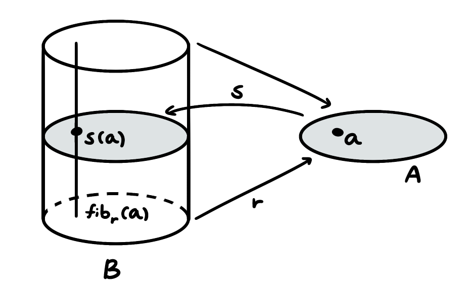
정의. 사상 $r: B \to A$과 $s: A \to B$가 $rs \sim \mathrm{id}_A$를 만족한다면 $s$를 $r$의 섹션이라고 하고, $r$을 $s$의 리트랙트라고 한다. 즉, 다음과 같이 정의한다.

\[\begin{gather} \mathrm{sec}(r) := \sum_{s': A \to B} rs' \sim \mathrm{id}_A\\ \mathrm{ret}(s) := \sum_{r': A \to B} r's \sim \mathrm{id}_B \end{gather}\]

정의. $B$가 $A$에 대한 유형족_{type family}이라고 하자. $x: A$가 주어졌을 때 $b(x): B(x)$라면, $b$를 $B$의 섹션이라고 부른다.

두 가지 의미의 섹션은 연관돼 있다. 첫 번째 정의를 기하학적으로 해석하면, 섹션 $s: A \to B$는 공간 $A$를 공간 $B$에 한 단면으로서 포함시키는 사상이며, 그에 대응되는 리트랙트 $r: B \to A$는 공간 $B$를 공간 $A$로 투영하는 사상이다. 이로부터 몇 가지 사실을 고찰할 수 있다.

• 일반적으로, “확대 후 축소”는 원 공간의 관계를 보존하지만 “축소 후 확대”는 보존하지 않는다. 이는 $r, s$가 리트랙트-섹션 관계일 때, $rs \sim \mathrm{id}_A$이지만 일반적으로 $sr \sim \mathrm{id}_B$이지는 않음을 시사한다.

• 섹션은 각 $a: A$에 대해 $r$의 $a$-섬유_fiber에서 한 점을 선택한다. 이는 도형의 $z$-등고면은 각각 특정한 $z$-좌푯값의 선택과 같은 것으로 이해할 수 있다.

• 그림에서 섬유는 한 가닥의 실처럼 보이며, 이것은 “섬유”라는 이름의 유래이다.

한편 $b$가 $A$에 대한 유형족 $B$의 섹션일 때, $b$는 각 $a: A$에 대해 $b(a): B(a)$를 선택한다. 여기서 $B(a)$는 $\mathrm{pr}_1: \sum_{x: A}B(x) \to A$의 $a$-섬유와 자연스럽게 동치이다. 따라서 $b$가 $B$의 (두 번째 의미에서의) 섹션일 때, $\lambda x. b(x)$는 $\mathrm{pr}_1$의 (첫 번째 의미에서의) 섹션이다.

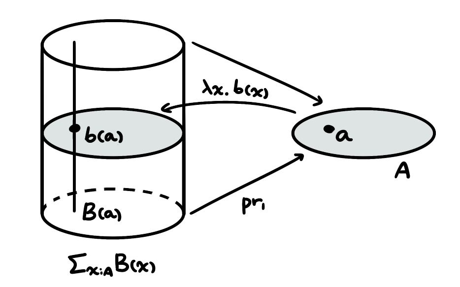
물론, $\lambda x . b(x)$는 $b$와 판단적으로 같다. 따라서 섹션의 두 번째 의미는 첫 번째 의미의 특수한 사례이다.

Notes on the Meaning of Sections

14 May 2026

In type theory, the term “section” appears in two different contexts.

Definition. Given maps $r: B \to A$ and $s: A \to B$, if $rs \sim \mathrm{id}_A$, then $s$ is called a section of $r$, and $r$ is called a retract of $s$. That is,

\[\begin{gather} \mathrm{sec}(r) := \sum_{s': A \to B} rs' \sim \mathrm{id}_A\\ \mathrm{ret}(s) := \sum_{r': A \to B} r's \sim \mathrm{id}_B \end{gather}\]

Definition. Let $B$ be a type family over $A$. Given $x: A$, if $b(x): B(x)$, then $b$ is called a section of $B$.

The two meanings of section are related. Regarding the first definition, geometrically, a section $s: A \to B$ is a map that includes the space $A$ as a (cross-)section in the space $B$, while the corresponding retract $r: B \to A$ is a map that projects the space $B$ onto the space $A$. From this, several observations can be made:

• Generally, “expanding and then contracting” preserves the relationship of the original space, but “contracting and then expanding” does not. This suggests that when $r$ and $s$ are in a retract-section relationship, $rs \sim \mathrm{id}_A$, but $sr \sim \mathrm{id}_B$ does not generally hold.

• A section chooses a point in the $a$-fibre of $r$ for each $a: A$. This can be understood as analogous to selecting a specific $z$-coordinate value for each $z$-contour of a figure.

• In the diagram, the fibre appears like a strand of thread, which is the origin of the term “fibre.”

On the other hand, when $b$ is a section of a type family $B$ over $A$, $b$ chooses $b(a): B(a)$ for each $a: A$. Here, $B(a)$ is naturally equivalent to the $a$-fibre of $\mathrm{pr}_1: \sum_{x: A}B(x) \to A$. Therefore, when $b$ is a section of $B$ (in the second sense), $\lambda x. b(x)$ is a section of $\mathrm{pr}_1$ (in the first sense).

Of course, $\lambda x . b(x)$ is judgementally equal to $b$. Thus, the second meaning of section is just a special case of the first.

유형론적 대각선 논법

13 May 2026

전사성의 유형론적 정의

정의. 사상 $f: A \to X$에 대해 다음과 같이 정의한다.

\[\text{is-surj}(f) := \prod_{x: X} \| \mathrm{fib}_f(x) \|\]

위의 정의는 “임의의 공역의 원소는 공집합이 아닌 역사상_fiber을 가진다”를 표현한 것이다. 이와 동치인 정의는 “공역이 치역과 같다”이다. 후자의 정의를 유형론적으로 옮기기 위해서 다음과 같이 정의한다.

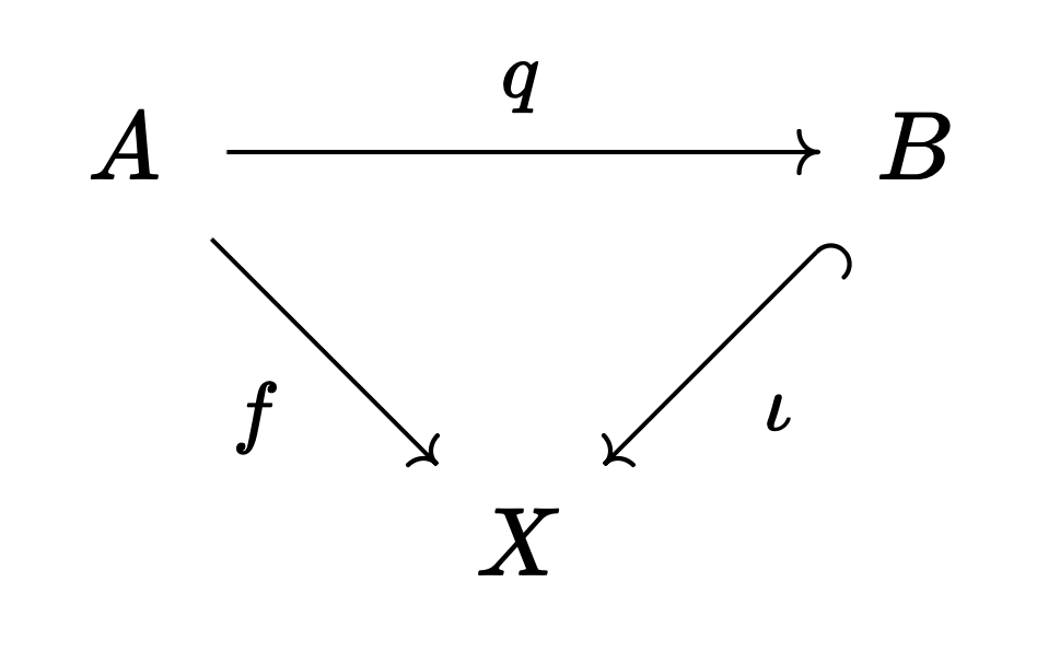
정의. 다음의 가환 도식에서 $\iota$가 임베딩이고, 가환성이 호모토피 $H: f \sim \iota q$에 의해 목격된다고 하자.

다음이 만족될 경우 $\iota$가 치역 임베딩의 보편 성질을 만족한다고 한다: 임의의 임베딩 $m: C \to X$에 대해, 전치 합성

\[- \circ (q, H): \hom_X(\iota, m) \to \hom_X(f, m)\]

이 동치 관계_equivalence이다.

위의 정의는 치역 임베딩의 보편 성질이 정말로 맞다. 즉, 다음이 성립한다.

정리. 사상 $f: A \to X$에 대해 다음이 성립한다.

• 다음은 치역 임베딩의 보편 성질을 만족한다.

\[\begin{align} &\operatorname{im} f := \sum_{x: X} \| \mathrm{fib}_f(x) \| \\ &q_f : A \to \operatorname{im} f; &&a \mapsto (f(a), |(a, \mathrm{refl}_{f(a)})) \\ &\iota_f : \operatorname{im} f \to X; &&\mathrm{pr}_1 \end{align}\]

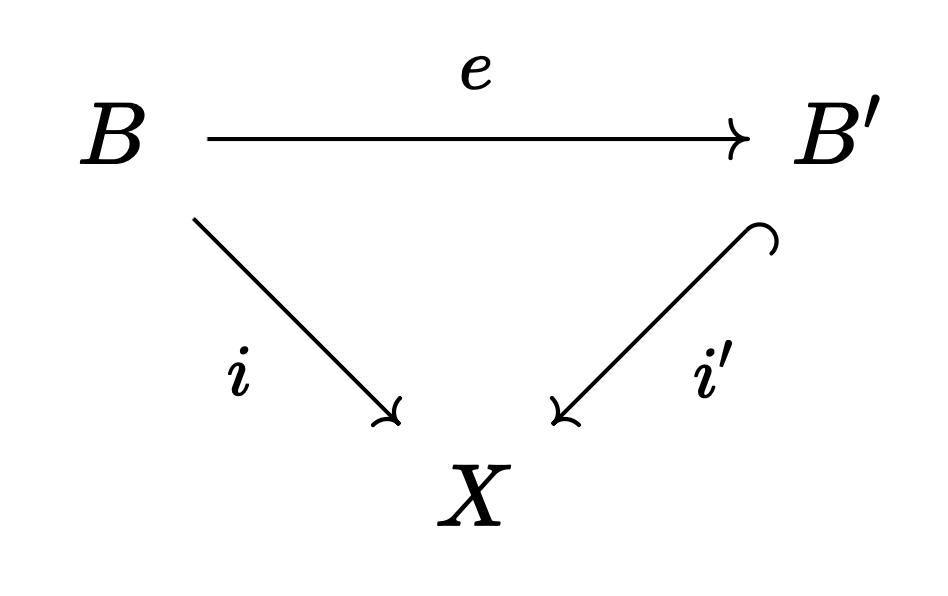
• 치역 임베딩의 보편 성질을 만족하는 임베딩은 유일하다. 즉, 두 임베딩 $i: B \to X$와 $i’: B’ \to X$가 보편 성질을 만족한다면, 다음의 가환 도식을 만족하는 동치 관계 $e: B \simeq B’$의 유형은 수축 가능하다_contractible.

유형론적으로 치역을 정의했으므로, 전사성의 두 번째 정의를 제시할 수 있다.

정리. 다음의 가환 도식에서 $\iota: B \to X$가 임베딩이라고 하자. $q$가 전사일 필요충분조건은 $\iota$가 치역 임베딩의 보편 성질을 만족하는 것이다.

유형론적 대각선 논법

정의. 유형 $X$에 대해, 다음과 같이 정의한다.

\[\mathcal{P}(X) := X \to \mathsf{Prop}\]

즉, $X$의 멱집합은 $X$에 대한 명제들의 모임_{family of propositions over $X$}이다. 이는 가령 자연수의 부분집합인 짝수 집합이 “짝수임”이라는 자연수에 대한 명제와 대응하는 것으로 이해할 수 있다. 한편, $X$의 멱집합을 $X \to 2$로 정의하지 않는 이유는 이 경우 $X$의 멱집합이 결정 가능한 명제로 한정되기 때문이다.

칸토어 정리. $f: X \to \mathcal{P}(X)$라면 $f$는 전사가 아니다.

증명. $X$에 대한 다음의 명제 $Q : X \to \mathsf{Prop}$를 정의하자.

\[Q := \lambda x. \lnot f(x, x)\]

$f$가 전사라면 $g: \prod_{P: X \to \mathsf{Prop}} \| \mathrm{fib}_f(P) \|$가 존재한다. 따라서 $g(Q) : \| \mathrm{fib}_f(Q) \|$이다.

다음과 같이 $\mathrm{fib}_f(Q) \to \varnothing$을 정의하자.

\[(x, p) \mapsto \mathrm{tr}(f(x, x), p)(f(x, x))\]

명제적 절단_{propositional truncation}의 정의로부터, 위의 사상은 $\| \mathrm{fib}_f(Q) \| \to \varnothing$을 유도한다. 따라서 $g(Q) \to \varnothing$이다. 이는 모순이므로 $f$는 전사가 아니다. ■

Type-Theoretic Diagonal Argument

13 May 2026

Type-Theoretic Definition of Surjectivity

Definition. For a map $f: A \to X$, we define:

\[\text{is-surj}(f) := \prod_{x: X} \| \mathrm{fib}_f(x) \|\]

The above definition expresses that “every element of the codomain has a non-empty fibre.” An equivalent definition is “the codomain equals the image.” To translate the latter definition into type theory, we define as follows:

Definition. Consider the following commutative diagram where $\iota$ is an embedding, and the commutativity is witnessed by a homotopy $H: f \sim \iota q$.

We say that $\iota$ satisfies the universal property of the image inclusion if the following holds: for any embedding $m: C \to X$, the precomposition

\[- \circ (q, H): \hom_X(\iota, m) \to \hom_X(f, m)\]

is an equivalence.

The above definition indeed satisfies the universal property of the image inclusion. That is, the following holds:

Theorem. For a map $f: A \to X$, the following holds:

• The following satisfies the universal property of the image inclusion:

\[\begin{align} &\operatorname{im} f := \sum_{x: X} \| \mathrm{fib}_f(x) \| \\ &q_f : A \to \operatorname{im} f; &&a \mapsto (f(a), |(a, \mathrm{refl}_{f(a)})) \\ &\iota_f : \operatorname{im} f \to X; &&\mathrm{pr}_1 \end{align}\]

• The embedding satisfying the universal property of the image inclusion is unique. That is, if two embeddings $i: B \to X$ and $i’: B’ \to X$ satisfy the universal property, then the type of equivalences $e: B \simeq B’$ satisfying the following commutative diagram is contractible.

Having defined the image type-theoretically, we can now present the second definition of surjectivity.

Theorem. In the following commutative diagram, let $\iota: B \to X$ be an embedding. Then $q$ is surjective if and only if $\iota$ satisfies the universal property of the image inclusion.

Type-Theoretic Diagonal Argument

Definition. For a type $X$, we define:

\[\mathcal{P}(X) := X \to \mathsf{Prop}\]

That is, the power set of $X$ is the family of propositions over $X$. For instance, the set of even natural numbers corresponds to the proposition “is even” over the natural numbers. On the other hand, the power set of $X$ is not defined as $X \to 2$ because, in this case, the power set of $X$ would be restricted to decidable propositions.

Cantor’s Theorem. For any $f: X \to \mathcal{P}(X)$, $f$ is not surjective.

Proof. Define the following proposition $Q : X \to \mathsf{Prop}$ over $X$:

\[Q := \lambda x. \lnot f(x, x)\]

If $f$ were surjective, then there would exist $g: \prod_{P: X \to \mathsf{Prop}} \| \mathrm{fib}_f(P) \|$. Hence, $g(Q) : \| \mathrm{fib}_f(Q) \|$.

Define $\mathrm{fib}_f(Q) \to \varnothing$ as follows:

\[(x, p) \mapsto \mathrm{tr}(f(x, x), p)(f(x, x))\]

From the definition of propositional truncation, the above map induces $\| \mathrm{fib}_f(Q) \| \to \varnothing$. Thus, $g(Q) \to \varnothing$, which is a contradiction. Therefore, $f$ is not surjective. ■

유형론적 요네다 보조정리

07 May 2026

요네다 보조정리. $\mathcal{A}$가 범주이고, $A \in \mathcal{A}$이며, $F: \mathcal{A}^\mathrm{op} \to \mathbf{Set}$이라고 하자. 다음의 동형 관계가 $A$와 $F$에서 자연스럽다.

\[[\mathrm{hom}_\mathcal{A}(-, A), F] \cong F(A)\]

이는 범주론의 잘 알려진 정리이다. 그런데 흥미롭게도, 요네다 보조정리와 비슷한 형태의 정리를 유형론에서 발견할 수 있다.

유형론적 요네다 보조정리. $A$가 유형이고, $B$가 $A$에 의존하는 유형이라고 하자. 각 $a : A$에 대해 다음이 성립한다.

\[\prod_{x: A}((x = a) \to B(x)) \simeq B(a)\]

둘의 유사성을 조금 더 부각하기 위해 기호를 바꿔 적으면 다음과 같다.

$\mathcal{A}$가 유형이고, $F$가 $\mathcal{A}$에 의존하는 유형이라고 하자. 각 $A : \mathcal{A}$에 대해 다음이 성립한다.

\[\prod_{X: \mathcal{A}}((X = A) \to F(X)) \simeq F(A)\]

유형론적 요네다 보조정리는 다음 정리의 특수한 사례이다.

정리. 각 $a: A$에 대해 다음 사상은 동형이다.

\[\mathrm{ev} : \prod_{x: A}\prod_{p: a = x} B(x, p) \to B(a, \mathrm{refl}_a); \quad h \mapsto h(a, \mathrm{refl}_a)\]

증명. 동일성 유형의 귀납법에 따라 다음 사상이 존재하며, $\mathrm{ev}$의 섹션이다.

\[\mathrm{ind} : B(a, \mathrm{refl}_a) \to \prod_{x: A}\prod_{p: a = x} B(x, p)\]

따라서 $\mathrm{ind}$가 $\mathrm{ev}$의 리트랙트라는 것을 보이면 충분하다. 즉, 각 $h: \prod_{x: A}\prod_{p: a = x} B(x, p)$에 대해 다음이 성립함을 보이면 충분하다.

\[\mathrm{ind}(h(a, \mathrm{refl}_a)) = h\]

함수 외연성 공리에 따라, 다음을 보이면 충분하다.

\[\prod_{x: A}\prod_{p: a = x} \mathrm{ind}(h(a, \mathrm{refl}_a), x, p) = h(x, p)\]

동일성 유형의 귀납법에 따라, 다음을 보이면 충분하다.

\[\mathrm{ind}(h(a, \mathrm{refl}_a), a, \mathrm{refl}_a) = h(a, \mathrm{refl}_a)\]

이는 $\mathrm{ind}$의 정의로부터 판단적으로 따라 나온다. ■

Type-Theoretic Yoneda Lemma

07 May 2026

Yoneda Lemma. Let $\mathcal{A}$ be a category, $A \in \mathcal{A}$, and $F: \mathcal{A}^\mathrm{op} \to \mathbf{Set}$. The following isomorphism is natural in $A$ and $F$:

\[[\mathrm{hom}_\mathcal{A}(-, A), F] \cong F(A)\]

This is a well-known theorem in category theory. Interestingly, a theorem similar in form to the Yoneda Lemma can also be found in type theory.

Type-Theoretic Yoneda Lemma. Let $A$ be a type, and let $B$ be a type dependent on $A$. For each $a : A$, the following holds:

\[\prod_{x: A}((x = a) \to B(x)) \simeq B(a)\]

To highlight the similarity between the two, we can rewrite the notation as follows:

Let $\mathcal{A}$ be a type, and let $F$ be a type dependent on $\mathcal{A}$. For each $A : \mathcal{A}$, the following holds:

\[\prod_{X: \mathcal{A}}((X = A) \to F(X)) \simeq F(A)\]

The type-theoretic Yoneda Lemma is a special case of the following theorem:

Theorem. For each $a: A$, the following map is an isomorphism:

\[\mathrm{ev} : \prod_{x: A}\prod_{p: a = x} B(x, p) \to B(a, \mathrm{refl}_a); \quad h \mapsto h(a, \mathrm{refl}_a)\]

Proof. By induction on the identity type, the following map exists and serves as a section of $\mathrm{ev}$:

\[\mathrm{ind} : B(a, \mathrm{refl}_a) \to \prod_{x: A}\prod_{p: a = x} B(x, p)\]

Thus, it suffices to show that $\mathrm{ind}$ is a retraction of $\mathrm{ev}$. That is, for each $h: \prod_{x: A}\prod_{p: a = x} B(x, p)$, we need to show:

\[\mathrm{ind}(h(a, \mathrm{refl}_a)) = h\]

By the principle of function extensionality, this amounts to showing:

\[\prod_{x: A}\prod_{p: a = x} \mathrm{ind}(h(a, \mathrm{refl}_a), x, p) = h(x, p)\]

By induction on the identity type, it suffices to show:

\[\mathrm{ind}(h(a, \mathrm{refl}_a), a, \mathrm{refl}_a) = h(a, \mathrm{refl}_a)\]

This follows judgmentally from the definition of $\mathrm{ind}$. ■

양자역학의 국소성에 대하여

23 Feb 2026

벨 부등식은 흔히 “양자역학은 국소적이지 않다”는 결론으로 요약되곤 한다. 그러나 이 요약은 오해를 일으키는 표현인데, 국소성의 표준적인 의미로 따지면 양자역학은 완벽히 국소적이기 때문이다. 국소성의 표준적 의미란 다음과 같다.

정의. 어떤 물리 이론이 국소적_local일 조건은, 시공간의 두 사건_event에 대해 한 사건이 다른 사건에 빛보다 빠르게 영향을 주지 않는 것이다.

그리고 위의 정의를 적절히 해석했을 때 양자역학은 국소적임을 증명할 수 있다. 가령, 두 개의 얽힌 입자 A와 B로 이루어진 계의 파동함수 $\psi(a, b)$를 생각하자. 만약 우리가 입자 A에만 관심을 가진다면, 입자 A를 대상으로 한 관측의 결과가 어떻게 나올지는 다음의 밀도 행렬_{density matrix}로 완전히 표현할 수 있다.

\[\rho_{a'a} = \sum_{b} \psi^*(a, b)\psi(a', b)\]

예를 들어 관측량_observable $\mathbf{L}$이 A에 국소적으로 작용할 때, $\mathbf{L}$의 기댓값은 다음과 같이 구할 수 있음이 알려져 있다.

\[\langle \mathbf{L} \rangle = \operatorname{tr} \rho L\]

여기서 $\mathbf{L}$이 A에 국소적으로 작용한다는 표현의 의미는 다음과 같다.

\[L_{a'b', ab} = L_{a'a} \delta_{b'b}\]

따라서 입자 B에서 국소적으로 일어나는 시간 변화가 입자 A의 밀도 행렬을 변화시키지 않는다면, 다음의 의미에서 양자역학은 국소적이다.

임의의 두 입자에 대해, 한 입자의 국소적 시간 변화가 다른 입자의 국소적 상태에 빛보다 빠르게 영향을 주지 않는다.

이 사실을 증명해 보자. 입자 B에서 국소적 시간 변화가 진행된다고 하자. 가령 입자 B의 위치를 관측하거나, 운동량을 관측하거나, 입자 B를 다른 입자와 얽히게 만드는 등의 일이 일어난다. 무슨 일이 일어나든 간에 이 일은 $\psi(a, b)$를 변화시킬 것이다. 양자역학에서 계의 시간에 따른 변화는 유니터리 행렬로 표현된다. 즉, 어떤 유니터리 연산자 $\mathbf{U}$가 존재하여, 일정 시간이 지난 이후 계의 상태를 $\psi_f(a’, b’)$라고 하면

\[\psi_f(a', b') = \sum_{a, b} U_{a'b', ab} \psi(a, b)\]

이다. 그런데 시간 변화가 B에서만 국소적으로 진행된다면 $a \neq a’$일 때 $U_{a’b’, ab} = 0$이다. 따라서,

\[\psi_f(a, b') = \sum_{b} U_{b'b} \psi(a, b)\]

로 줄여 쓸 수 있다. 이로 인해 A의 밀도 행렬은 다음과 같이 갱신된다.

\[\rho'_{a'a} = \sum_{b} \psi_f^*(a, b)\psi(a', b)\]

두 식을 연립하면,

\[\begin{align} \rho'_{a'a} &= \sum_{b} \left( \left( \sum_{b'} U_{bb'} \psi(a, b') \right)^* \left( \sum_{b''} U_{bb''} \psi(a', b'') \right) \right) \\ &= \sum_{b, b', b''} U^*_{b'b} U_{bb''} \psi^*(a, b') \psi(a', b'') \end{align}\]

이다. 그런데 $\mathbf{U}$가 유니터리이므로 $\sum_b U^\ast_{b’b} U_{bb’’} = (U^\ast U)_{b’ b’’} = \delta_{b’ b’’}$이다. 따라서,

\[\rho'_{a'a} = \sum_{b'} \psi^*(a, b') \psi(a', b') = \rho_{a'a}\]

이다. 따라서 $\rho’ = \rho$이다. 즉, B에서 국소적으로 진행되는 유니터리한 시간 변화는 A의 밀도 행렬을 변화시키지 않는다. 실질적으로 이는 다음의 정리를 증명한 것이다.

통신 없음 정리_{No-communication theorem}. (얽힘을 고려하더라도) 빛보다 빠르게 정보를 전달하는 것은 불가능하다.

그렇다면 벨 부등식을 비롯한, 흔히 양자역학의 비국소성을 보여주는 것으로 제시되는 사례들은 어떻게 이해되어야 하는가? 가령, 코펜하겐 해석에 따르면 각운동량의 총합이 0인 두 전자를 앨리스와 밥이 나눠가진 뒤, 밥이 스핀 업의 전자를 관측한다면, 앨리스의 전자는 그 즉시 스핀 다운으로 붕괴된다. 그렇다면 앨리스의 전자의 밀도 행렬도 그에 맞추어 변해야 하는 것 아닌가?

이 질문에 대한 “실증주의적” 해답은 이렇다 (실증주의적이라는 표현은 이 해답에 대한 철학적 해석을 일단 차치하겠다는 것이다). 만약 두 개의 전자뿐 아니라 앨리스와 밥 또한 전체 계의 일부로 간주한다면, 밥의 관측이 있기 전과 후 계의 파동함수는 다음과 변화한다.

관측 전:

\[\begin{align} \psi &= \frac{1}{\sqrt{2}}(\text{Alice has not observed her spin-up electron}\\ &\qquad \land \,\,\, \text{Bob has not observed his spin-down electron}) \\ &+ \frac{1}{\sqrt{2}}(\text{Alice has not observed her spin-down electron} \\ &\qquad \land \,\,\, \text{Bob has not observed his spin-up electron}) \end{align}\]

관측 후:

\[\begin{align} \psi_f &= \frac{1}{\sqrt{2}}(\text{Alice has not observed her spin-up electron}\\ &\qquad \land \,\,\, \text{Bob has observed his spin-down electron}) \\ &+ \frac{1}{\sqrt{2}}(\text{Alice has not observed her spin-down electron} \\ &\qquad \land \,\,\, \text{Bob has observed his spin-up electron}) \end{align}\]

즉, 밥도 계의 일부이기 때문에 밥의 행위는 계를 불연속적으로 붕괴시키는 것이 아닌, 계의 유니터리한 시간 변화의 일부이다. 대신 앨리스-밥 계의 외부에서 제3자인 찰리가 밥을 관측한다면 그때는 $\psi_f$가 가령 다음과 같이 붕괴할 것이다.

\[\begin{align} \psi_f \longmapsto\; &(\text{Alice has not observed her spin-down electron} \\ &\land \; \text{Bob has observed his spin-up electron}) \end{align}\]

그러나 만약 찰리 또한 밥과 앨리스와 함께 계의 일부로 간주한다면, 전체 계의 파동함수는 다음과 같이 유니터리하게 시간 변화한다.

\[\begin{align} \psi_f &= \frac{1}{\sqrt{2}}(\text{Alice has not observed her spin-up electron}\\ &\qquad \land \,\,\, \text{Bob has observed his spin-down electron} \\ &\qquad \land \,\,\, \text{Charlie has observed Bob observing spin-down}) \\ &+ \frac{1}{\sqrt{2}}(\text{Alice has not observed her spin-down electron} \\ &\qquad \land \,\,\, \text{Bob has observed his spin-up electron} \\ &\qquad \land \,\,\, \text{Charlie has observed Bob observing spin-up}) \\ \end{align}\]

일반적으로, 관측자와 계를 분리하면 관측은 계의 파동함수를 붕괴시키지만, 관측자를 계에 포함시키면 관측 또한 계의 유니터리 시간 변화의 일부이다. 이 결론을 확장하면, 우주 전체의 파동함수는 항상 유니터리하게 시간 변화하며, 우주 전체의 파동함수만이 유일하게 물리적으로 유의미한 파동함수라는 주장을 얻는다. 이는 양자역학에 대한 다세계 해석으로 이어지게 된다.

On the Locality of Quantum Mechanics

23 Feb 2026

This post was originally written in Korean, and has been machine translated into English. It may contain minor errors or unnatural expressions. Proofreading will be done in the near future.

The Bell inequality is often summarised as concluding that “quantum mechanics is non-local.” However, this summary is misleading, as quantum mechanics is perfectly local when judged by the standard definition of locality. The standard definition of locality is as follows:

Definition. A physical theory is local if, for any two events in spacetime, one event does not influence the other faster than the speed of light.

When interpreted appropriately, quantum mechanics can be shown to be local under this definition. For instance, consider a system consisting of two entangled particles, A and B, with a wavefunction $\psi(a, b)$. If we are only interested in particle A, the outcomes of measurements on A can be fully described by the following density matrix:

\[\rho_{a'a} = \sum_{b} \psi^*(a, b)\psi(a', b)\]

For example, when an observable $\mathbf{L}$ acts locally on A, the expectation value of $\mathbf{L}$ is known to be given by:

\[\langle \mathbf{L} \rangle = \operatorname{tr} \rho L\]

Here, the expression “observable $\mathbf{L}$ acts locally on A” means the following:

\[L_{a'b', ab} = L_{a'a} \delta_{b'b}\]

Thus, if local changes in time at particle B do not affect the density matrix of particle A, quantum mechanics is local in the following sense:

For any two particles, local changes in time at one particle do not influence the local state of the other particle faster than the speed of light.

Let us prove this. Suppose a local change in time occurs at particle B, such as measuring its position, momentum, or entangling it with another particle. Whatever happens, this will alter $\psi(a, b)$. In quantum mechanics, the time evolution of a system is represented by a unitary matrix. That is, there exists a unitary operator $\mathbf{U}$ such that, after some time, the state of the system becomes $\psi_f(a’, b’)$:

\[\psi_f(a', b') = \sum_{a, b} U_{a'b', ab} \psi(a, b)\]

If the time evolution is local to B, then $U_{a’b’, ab} = 0$ when $a \neq a’$. Hence,

\[\psi_f(a, b') = \sum_{b} U_{b'b} \psi(a, b)\]

This leads to the following update of A’s density matrix:

\[\rho'_{a'a} = \sum_{b} \psi_f^*(a, b)\psi(a', b)\]

Combining the two equations, we have:

\[\begin{align} \rho'_{a'a} &= \sum_{b} \left( \left( \sum_{b'} U_{bb'} \psi(a, b') \right)^* \left( \sum_{b''} U_{bb''} \psi(a', b'') \right) \right) \\ &= \sum_{b, b', b''} U^*_{b'b} U_{bb''} \psi^*(a, b') \psi(a', b'') \end{align}\]

Since $\mathbf{U}$ is unitary, $\sum_b U^\ast_{b’b} U_{bb’’} = (U^\ast U)_{b’ b’’} = \delta_{b’ b’’}$. Therefore,

\[\rho'_{a'a} = \sum_{b'} \psi^*(a, b') \psi(a', b') = \rho_{a'a}\]

Thus, $\rho’ = \rho$. In other words, unitary time evolution local to B does not alter the density matrix of A. This effectively proves the following theorem:

No-communication theorem. (Even considering entanglement) It is impossible to transmit information faster than the speed of light.

How, then, should we understand cases like the Bell inequality, which are often presented as evidence of the non-locality of quantum mechanics? For instance, according to the Copenhagen interpretation, if Alice and Bob share two electrons with a total angular momentum of zero, and Bob observes a spin-up electron, Alice’s electron instantaneously collapses to spin-down. Does this not imply that Alice’s electron’s density matrix changes accordingly?

The “positivist” answer to this question is as follows (the term “positivist” is used here to set aside philosophical interpretations for now). If not only the two electrons but also Alice and Bob are considered part of the entire system, the wavefunction of the system evolves as follows before and after Bob’s observation:

Before observation:

\[\begin{align} \psi &= \frac{1}{\sqrt{2}}(\text{Alice has not observed her spin-up electron}\\ &\qquad \land \,\,\, \text{Bob has not observed his spin-down electron}) \\ &+ \frac{1}{\sqrt{2}}(\text{Alice has not observed her spin-down electron} \\ &\qquad \land \,\,\, \text{Bob has not observed his spin-up electron}) \end{align}\]

After observation:

\[\begin{align} \psi_f &= \frac{1}{\sqrt{2}}(\text{Alice has not observed her spin-up electron}\\ &\qquad \land \,\,\, \text{Bob has observed his spin-down electron}) \\ &+ \frac{1}{\sqrt{2}}(\text{Alice has not observed her spin-down electron} \\ &\qquad \land \,\,\, \text{Bob has observed his spin-up electron}) \end{align}\]

In other words, since Bob is part of the system, his actions are not a discontinuous collapse of the system but part of its unitary time evolution. Instead, if a third party, Charlie, observes Bob, then $\psi_f$ might collapse as follows:

\[\begin{align} \psi_f \longmapsto\; &(\text{Alice has not observed her spin-down electron} \\ &\land \; \text{Bob has observed his spin-up electron}) \end{align}\]

However, if Charlie is also considered part of the system along with Bob and Alice, the wavefunction of the entire system evolves unitarily as follows:

\[\begin{align} \psi_f &= \frac{1}{\sqrt{2}}(\text{Alice has not observed her spin-up electron}\\ &\qquad \land \,\,\, \text{Bob has observed his spin-down electron} \\ &\qquad \land \,\,\, \text{Charlie has observed Bob observing spin-down}) \\ &+ \frac{1}{\sqrt{2}}(\text{Alice has not observed her spin-down electron} \\ &\qquad \land \,\,\, \text{Bob has observed his spin-up electron} \\ &\qquad \land \,\,\, \text{Charlie has observed Bob observing spin-up}) \\ \end{align}\]

In general, if the observer and the system are separated, observation collapses the system’s wavefunction, but if the observer is included in the system, observation is part of the system’s unitary time evolution. Extending this conclusion, the wavefunction of the entire universe always evolves unitarily, and only the wavefunction of the entire universe is physically meaningful. This leads to the many-worlds interpretation of quantum mechanics.