디멘의 블로그 Jeongdam's Blog
교환법칙, 분배법칙, 지수법칙의 범주론적 증명
27 Dec 2025정리.
- 분배법칙: $(A + B) \times C = A \times C + B \times C$
- 지수법칙: $(A \times B)^C = A^C \times B^C$
이전 글에서 범주론적 합과 곱을 살펴 보았다. 합은 쌍극한의 일종이고, 곱은 극한의 일종이다. 이 관찰로부터, 분배법칙과 지수법칙을 다음 정리로 일반화할 수 있다.
정리. 좌 어드조인트는 쌍극한colimit을, 우 어드조인트는 극한limit을 보존한다.
이 정리의 정확한 의미는 다음과 같다. $F: \mathcal{A} \to \mathcal{B}, G: \mathcal{B} \to \mathcal{A}$에 대해 $F \dashv G$라고 하자. $G$가 극한을 보존preserves limits한다는 것은, 임의의 작은 범주small category $\mathbf{I}$와 함자 $D : \mathbf{I} \to \mathcal{B}$에 대해 다음이 성립한다는 것이다.
$\big(B \xrightarrow{q_I} D(I)\big)_{I \in \mathbf{I}}$가 $\mathcal{B}$에서 극한 고깔limit cone일 때, $\big(G(B) \xrightarrow{G(q_I)} GD(I)\big)_{I \in \mathbf{I}}$가 $\mathcal{A}$에서 극한 고깔이다.
이로부터, $G$가 극한을 보존할 때 다음이 성립함을 알 수 있다.
\[G\left(\lim_{\leftarrow \mathbf{I}} D\right) \cong \lim_{\leftarrow \mathbf{I}} G \circ D\]쌍극한의 경우에는 고깔을 쌍고깔로 바꿔 정의한다.
한편, 임의의 $X, Y, Z \in \mathbf{Set}$에 대해 $\hom(X \times Y, Z) \cong \hom(X, Z^Y)$가 성립한다 (이는 함수형 프로그래밍에서 자주 등장하는 커링Currying 기법이다). 이로부터 다음의 어드조인트 관계가 따라 나온다.
\[(-) \times Y \dashv (-)^Y\]따라서 함자 $(-) \times Y$는 쌍극한을 보존하고, $(-)^Y$는 극한을 보존한다. 이로부터 일반화된 분배법칙과 지수법칙을 얻을 수 있다.
정리. 집합 $A, B, Y$에 대해, $A, B$가 서로소라면 다음이 성립한다.
- $(A + B) \times Y \cong (A \times Y) + (B \times Y)$
- $(A \times B)^Y \cong A^Y \times B^Y$
여기서 $+$는 서로소 집합의 합집합으로, $\sqcup$과 의미가 같으나 분배법칙과의 유사성을 강조하기 위해 사용되었다. 좌변이 $G\left(\lim_{\leftarrow \mathbf{I}} D\right)$에, 우변이 $\lim_{\leftarrow \mathbf{I}} G \circ D$에 대응된다. 위 정리에 집합의 크기 연산을 취하면 자연수에서의 분배법칙과 지수법칙을 얻는다.
참고로 극한에 대한 다음 성질 또한 알려져 있다 ($\bullet, -$ 표기법은 이 글을 참고)
정리. $\mathbf{I}, \mathbf{J}$가 작은 범주이고, $\mathcal{S}$가 $\mathbf{I}, \mathbf{J}$ 모양의 극한들을 가지는 국소적으로 작은 범주라고 하자. $D: \mathbf{I} \times \mathbf{J} \to \mathcal{S}$에 대해, 다음이 성립한다.
\[\lim_{\leftarrow \mathbf{J}}\lim_{\leftarrow \mathbf{I}} D(\bullet, -) \cong \lim_{\leftarrow \mathbf{I} \times \mathbf{J}} D \cong \lim_{\leftarrow \mathbf{I}}\lim_{\leftarrow \mathbf{J}} D(-, \bullet)\]
즉, 극한끼리는 교환법칙을 만족한다. 이것은 덧셈의 교환법칙과 곱셈의 교환법칙을 일반화한 것으로 생각할 수 있다.
Categorical Proofs of the Commutative Law, Distributive Law, and Exponential Law
27 Dec 2025This post was originally written in Korean, and has been machine translated into English. It may contain minor errors or unnatural expressions. Proofreading will be done in the near future.
Theorem.
- Distributive law: $(A + B) \times C = A \times C + B \times C$
- Exponential law: $(A \times B)^C = A^C \times B^C$
In a previous post, we explored categorical sums and products. Sums are a type of colimit, while products are a type of limit. From this observation, the distributive and exponential laws can be generalised into the following theorem.
Theorem. Left adjoints preserve colimits, and right adjoints preserve limits.
The precise meaning of this theorem is as follows. Let $F: \mathcal{A} \to \mathcal{B}$ and $G: \mathcal{B} \to \mathcal{A}$, and suppose $F \dashv G$. The statement that $G$ preserves limits means that for any small category $\mathbf{I}$ and functor $D : \mathbf{I} \to \mathcal{B}$, the following holds:
If $\big(B \xrightarrow{q_I} D(I)\big)_{I \in \mathbf{I}}$ is a limit cone in $\mathcal{B}$, then $\big(G(B) \xrightarrow{G(q_I)} G(D(I))\big)_{I \in \mathbf{I}}$ is a limit cone in $\mathcal{A}$.
From this, we can deduce the following when $G$ preserves limits:
\[G\left(\lim_{\leftarrow \mathbf{I}} D\right) \cong \lim_{\leftarrow \mathbf{I}} G \circ D\]For colimits, the definition is analogous, replacing cones with cocones.
On the other hand, for any $X, Y, Z \in \mathbf{Set}$, the following holds: $\hom(X \times Y, Z) \cong \hom(X, Z^Y)$ (this is a common technique in functional programming known as currying). From this, the following adjoint relationship arises:
\[(-) \times Y \dashv (-)^Y\]Thus, the functor $(-) \times Y$ preserves colimits, and the functor $(-)^Y$ preserves limits. From this, we can derive the generalised distributive and exponential laws.
Theorem. For sets $A, B, Y$, if $A$ and $B$ are disjoint, the following holds:
- $(A + B) \times Y \cong (A \times Y) + (B \times Y)$
- $(A \times B)^Y \cong A^Y \times B^Y$
Here, $+$ denotes the disjoint union of sets, which is equivalent to $\sqcup$, but the notation $+$ is used to emphasise its similarity to the distributive law. The left-hand side corresponds to $G\left(\lim_{\leftarrow \mathbf{I}} D\right)$, while the right-hand side corresponds to $\lim_{\leftarrow \mathbf{I}} G \circ D$. By applying cardinality operations to the sets in the above theorem, we recover the distributive and exponential laws for natural numbers.
Additionally, the following property of limits is also known (the $\bullet, -$ notation is explained in this post):
Theorem. Let $\mathbf{I}$ and $\mathbf{J}$ be small categories, and let $\mathcal{S}$ be a locally small category that admits limits of shape $\mathbf{I}$ and $\mathbf{J}$. For $D: \mathbf{I} \times \mathbf{J} \to \mathcal{S}$, the following holds:
\[\lim_{\leftarrow \mathbf{J}}\lim_{\leftarrow \mathbf{I}} D(\bullet, -) \cong \lim_{\leftarrow \mathbf{I} \times \mathbf{J}} D \cong \lim_{\leftarrow \mathbf{I}}\lim_{\leftarrow \mathbf{J}} D(-, \bullet)\]
In other words, limits satisfy the commutative law. This can be thought of as a generalisation of the commutative laws for addition and multiplication.
서슬린의 문제와 다이아몬드 원리
26 Dec 2025이전 글에서 다음 정리를 소개했다.
집합론적 실수의 정의. 다음을 만족하는 순서 집합 $(R, <)$은 순서 동형에 대해 유일하다.
- 완비 전순서 집합이다.
- 양끝점이 없다.
- 분리 가능separable하다. 즉, 어떤 가산인 $Q \subset R$이 존재하여 $Q$가 $R$에서 조밀dense하다.
3번 성질로부터 다음이 따라 나온다.
정리. $\mathcal{C}$가 $\mathbb{R}$의 개구간들의 모임이라고 하자. $\mathcal{C}$의 원소들이 쌍으로 서로소pairwise disjoint라면 $\mathcal{C}$는 가산이다.
증명. $\mathcal{C}$의 원소들이 쌍으로 서로소이므로, 각 $(x, y) \in \mathcal{C}$를 $q \in (x, y) \cap \mathbb{Q}$에 대응시키는 단사 사상 $\mathcal{C} \to \mathbb{Q}$가 존재한다. 따라서 $\mathcal{C}$는 가산이다. ■
쌍으로 서로소인 개구간들의 모임이 기껏 가산인 순서 집합은 가산 체인 성질countable chain condition을 가진다고 한다. 이 특이한 이름의 이유는 뒤에서 설명할 것이다.
서슬린의 문제Suslin’s problem는 집합론적 실수의 정의에서 분리 가능성을 가산 체인 성질로 약화시킬 수 있는지를 묻는다.
정의. 양끝점이 없고 가산 체인 성질을 가지는 완비 전순서 집합 중 실수와 순서 동형이 아닌 순서 집합을 서슬린 선Suslin line이라고 한다.
따라서 서슬린 선은 분리 가능하지 않아야 한다.
서슬린의 문제. 서슬린 선이 존재하는가?
1920년에 제기된 이 문제는, 1971년 솔로베이Solovay와 테넨바움Tennenbaum에 의해 ZFC와 독립적임이 증명되었다. 이 글에서는 독립성 증명을 살펴보는 대신, 서슬린 선의 조합론적 버전인 서슬린 트리에 대해서 알아보고자 한다. 우선 다음의 유명한 정리를 보자.
쾨니히 보조정리König’s lemma. 트리 $T$에 대해, $T$의 높이가 $\omega$이고, $T$의 각 노드가 유한한 수의 자식을 가진다면, $T$는 길이가 $\omega$인 가지를 가진다.
증명. $\alpha_0$를 루트 노드라고 하고, 다음과 같이 귀납적으로 노드열을 정의한다. $\alpha_n$이 주어졌을 때, $\alpha_n$의 자식 노드의 수는 유한하므로, 어떤 자식 노드에 대해 해당 노드를 루트로 하는 트리는 높이가 무한하다. 그러한 자식 노드 중 하나를 선택하여 (여기서 선택 공리가 필요하다) $\alpha_{n + 1}$로 정의한다. $\lbrace a_n \rbrace $은 길이가 무한한 가지이다. ■
$T$의 노드가 가산 수의 자식을 가질 수 있다면 다음과 같이 $T$의 모든 가지가 유한 길이임에도 $T$의 높이는 $\omega$일 수 있다.
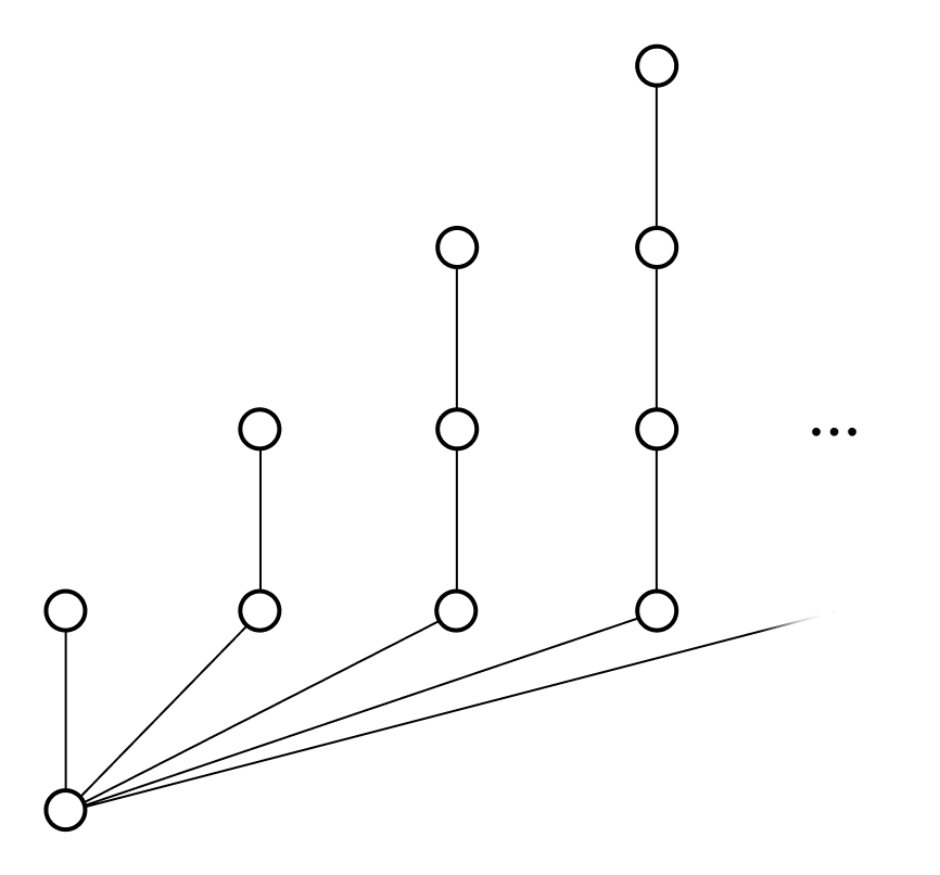
자연스러운 질문은, 쾨니히 보조정리를 비가산 기수에 대해 확장할 수 있는지이다. 그러나 이 질문에 대한 답은 부정적이다.
아론샤인 정리Aronszajn theorem. 높이가 $\omega_1$이고, 각 노드가 가산 수의 자식을 가지지만, 길이가 $\omega_1$인 가지가 없는 트리가 존재한다. (그러한 트리를 높이 $\omega_1$의 아론샤인 트리라고 한다.)
따라서 쾨니히 보조정리를 비가산 기수로 확장하기 위해서는 “각 노드가 가산 수의 자식을 가진다”보다 더 강력한 조건이 필요하다. 이를 위해 다음의 정의를 도입한다.
정의. 트리 $T$의 부분집합 $S$에 대해, $S$의 원소들이 서로 비교 불가능mutually incomparable할 때, $S$를 반체인antichain이라고 한다. $T$의 모든 반체인이 가산일 때, $T$가 가산 체인 성질을 가진다고 한다.
예를 들어 다음 트리의 색칠된 노드들은 반체인을 이룬다.
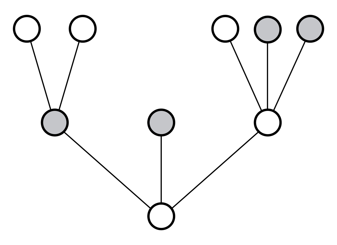
“각 노드가 가산 수의 자식을 가진다”가 국소적 성질이라면, 가산 체인 성질은 트리 전체에 관한 전역적 성질이다. 즉, 가산 체인 성질은 직관적으로 트리의 “너비”가 $\omega_1$보다 작다는 의미이다. 참고로 가산 반체인 성질이 아니라 가산 체인 성질이라고 부르는 것은 역사적 이유이기 때문에 크게 신경 쓸 필요는 없다.
앞서 쌍으로 서로소인 실수의 개구간들의 모임이 기껏 가산인 성질 또한 가산 체인 성질이라고 부른다고 했는데, 두 용법은 밀접한 관련이 있다. 반체인의 일반적인 정의는 다음과 같다.
정의. $(P, \leq)$가 부분순서라고 하자. $x, y \in P$가 비교 불가능하다는 것은, $z \leq x, z \leq y$인 $z \in P$가 존재하지 않는다는 것이다. $S \subseteq P$의 원소들이 서로 비교 불가능할 때 $S$를 반체인이라고 한다. $P$의 모든 반체인이 가산일 때, $P$가 가산 체인 성질을 가진다고 한다.
트리 $T$에서, 노드 $x$가 노드 $y$의 후손일 때 $x \leq y$라고 하자. 이때 트리의 노드로서 $x, y$가 비교 불가능한 것은 $(T, \leq)$의 원소로서 $x, y$가 비교 불가능한 것과 동치이다.
정의. 가산 체인 성질을 가지는 아론샤인 트리를 서슬린 트리라고 한다.
서슬린 트리의 존재성은 서슬린 선의 존재성과 동치이기 때문에 ZFC와 독립적이다. 동치가 되는 개략적인 이유는 각 성질이 다음 표와 같이 대응하기 때문이다.
| 서슬린 선 | 서슬린 트리 |
|---|---|
| 분리 불가능성 | 트리의 높이가 $\omega_1$ |
| 개구간의 가산 체인 성질 | 트리의 가산 체인 성질 |
분리 불가능성이 높이 $\omega_1$ 성질에 대응되는 개략적인 이유는, 어떤 집합 $D$가 존재하여 $|D| \leq \aleph_0$이고 임의의 개구간 $(a, b)$가 $D$와 교차한다는 사실이 (분리 가능성), 어떤 서수 $\alpha$가 존재하여 $\alpha < \omega_1$이고 임의의 노드 $x \in T$에 대해 $x$가 $T^{(\alpha)}$의 노드들로 이루어진 노드열의 극한이라는 사실과 (트리의 높이가 가산) 대응되기 때문이다.
서슬린 트리와 관련하여, 집합론의 다음 비표준 공리를 살펴보자.
다이아몬드 원리. 어떤 집합열 $\langle W_\alpha : \alpha < \omega_1 \rangle$가 존재하여 $W_\alpha \subseteq \mathcal{P}(\alpha)$이고, 각 $W_\alpha$가 가산집합이며, 임의의 $X \subseteq \omega_1$에 대해 $\lbrace \alpha : \alpha < \omega_1, X \cap \alpha \in W_\alpha \rbrace $가 정상 집합stationary set이다.
다이아몬드 원리는 $\Diamond$로 자주 표기한다. 또한 다이아몬드 원리의 $\langle W_\alpha \rangle$을 다이아몬드 열이라고 부른다.
$X \cap \alpha$는 $\alpha$라는 “거울”을 통해 “비춰” 보인 $X$의 모습으로 생각될 수 있다. 이 경우, 다이아몬드 원리는 $\omega_1$보다 작은 서수들에서 $X$의 반사된 모습이 $\langle W_\alpha \rangle$에서 충분히 자주 나타난다는 의미로 이해될 수 있다 (이 글에서 정상 집합이 “측도 > 0”의 집합론적 버전임을 설명했다).
따라서 다이아몬드 원리는 반사 원리reflection principle의 일종이며, $V = L$ 공리와 비슷하게 집합론적 우주를 규제하는 역할을 한다 (실제로 $V = L$은 $\Diamond$를 함의한다). 그리고 집합론적 우주를 규제하는 공리들이 그렇듯이, 다이아몬드 원리는 연속체 가설을 함의한다.
정리. $\Diamond \implies \mathsf{CH}$
증명. $X \subseteq \omega \subset \omega_1$이라고 하자. $X$가 $< \omega_1$에서 정상적으로 반사되므로, 어떤 $\alpha > \omega$에 대해 $X \cap \alpha = X \in W_\alpha$이다. 따라서 $\omega$의 부분집합들은 모두 $\bigcup_{\alpha < \omega_1} W_\alpha$에 속하는데, 후자의 기수가 $\aleph_1$이므로 $2^{\aleph_0} = \aleph_1$이다. ■
정리. $\Diamond$라면 서슬린 선이 존재한다.
증명. Hrbacek & Jech (3rd ed), Chapter 12, Section 5를 참고하라. 참고로 원문에는 다음의 오타가 있으니 주의하라.
(원문) Lemma 5.3. $\Diamond$ implies that there exists a sequence $\langle Z_\alpha : \alpha < \omega_1 \rangle$ such that, for each $\alpha < \omega_1$, $Z_\alpha \subseteq \omega^{<\alpha}$, $Z_\alpha$ is at most countable, and for any $X \subseteq \omega^{<\omega_1}$ the set $\lbrace \alpha < \omega_1 : X \cap \omega^{<\alpha} \rbrace $ is stationary.
Proof. We note that […] Clearly, $Z_\alpha \subseteq \omega^{<\alpha}$ and is at most countable.
(수정) Lemma 5.3. $\Diamond$ implies that there exists a sequence $\langle Z_\alpha : \alpha < \omega_1 \rangle$ such that, for each $\alpha < \omega_1$, $Z_\alpha \subseteq \mathcal{P}(\omega^{<\alpha})$, $Z_\alpha$ is at most countable, and for any $X \subseteq \omega^{<\omega_1}$ the set $\lbrace \alpha < \omega_1 : X \cap \omega^{<\alpha} \rbrace $ is stationary.
Proof. We note that […] Clearly, $Z_\alpha \subseteq \mathcal{P}(\omega^{<\alpha})$ and is at most countable.
또한 Claim 5.5 직전에 나오는 문장 “Let $\lbrace C_n : n \in \mathbb{N} \rbrace $ be the at most countable collection of those elements of $Z_\alpha$ which happen to be maximal antichains in $T^{(\alpha)}$.”의 의미는, 각 $n$에 대해 $C_n \in Z_\alpha$이고, $C_n \subseteq \omega^\alpha$이며, $C_n$의 원소들을 $T^{(\alpha)}$의 노드로 간주했을 때 $C_n$이 반체인이라는 것이다. ■
따름정리. $V = L$이라면 서슬린 선이 존재한다.
따라서 서슬린 선의 존재성은 집합론적 우주의 규제와 관련이 있다. 이 사실이 모순적으로 느껴질 수 있지만, 서슬린 선의 조건 중 하나가 가산 조밀 집합의 “비”존재라는 사실을 고려하면 그렇게 이상한 것은 아니다. 서슬린 선은 가산 체인 성질까지만 얻고 가산 조밀 집합은 발생시키지 않는 것이 가능한 “허술한” 집합론적 우주의 특징인 것이다.
Suslin's Problem and the Diamond Principle
26 Dec 2025This post was originally written in Korean, and has been machine translated into English. It may contain minor errors or unnatural expressions. Proofreading will be done in the near future.
In the previous post, the following theorem was introduced:
Definition of the set-theoretic real numbers. A totally ordered set $(R, <)$ satisfying the following properties is unique up to order isomorphism:
- It is a complete totally ordered set.
- It has no endpoints.
- It is separable, i.e., there exists a countable $Q \subset R$ such that $Q$ is dense in $R$.
From the third property, the following result follows:
Theorem. Let $\mathcal{C}$ be the collection of open intervals of $\mathbb{R}$. If the elements of $\mathcal{C}$ are pairwise disjoint, then $\mathcal{C}$ is countable.
Proof. Since the elements of $\mathcal{C}$ are pairwise disjoint, there exists an injective mapping $\mathcal{C} \to \mathbb{Q}$ that maps each $(x, y) \in \mathcal{C}$ to some $q \in (x, y) \cap \mathbb{Q}$. Hence, $\mathcal{C}$ is countable. ■
A totally ordered set in which any collection of pairwise disjoint open intervals is at most countable is said to have the countable chain condition. The peculiar name of this property will be explained later.
Suslin’s problem asks whether the separability condition in the definition of the set-theoretic real numbers can be weakened to the countable chain condition.
Definition. A complete totally ordered set without endpoints that satisfies the countable chain condition but is not order-isomorphic to the real numbers is called a Suslin line.
Thus, a Suslin line must not be separable.
Suslin’s problem. Does a Suslin line exist?
This problem, posed in 1920, was shown to be independent of ZFC by Solovay and Tennenbaum in 1971. Instead of examining the independence proof, this post will explore the combinatorial counterpart of Suslin lines, known as Suslin trees. Let us first consider the following well-known theorem:
König’s lemma. For a tree $T$, if $T$ has height $\omega$ and each node has finitely many children, then $T$ has a branch of length $\omega$.
Proof. Let $\alpha_0$ be the root node, and define a sequence of nodes inductively as follows. Given $\alpha_n$, since $\alpha_n$ has finitely many children, there exists a child node such that the subtree rooted at that node has infinite height. Choose one such child node (using the axiom of choice) and define it as $\alpha_{n+1}$. The sequence ${a_n}$ forms a branch of infinite length. ■
If the nodes of $T$ are allowed to have countably many children, it is possible for all branches of $T$ to have finite length while $T$ itself has height $\omega$, as illustrated below:
A natural question is whether König’s lemma can be extended to uncountable cardinals. However, the answer to this question is negative.
Aronszajn’s theorem. There exists a tree of height $\omega_1$ in which each node has countably many children, but no branch has length $\omega_1$. (Such a tree is called an Aronszajn tree of height $\omega_1$.)
Thus, to extend König’s lemma to uncountable cardinals, a stronger condition than “each node has countably many children” is required. To this end, the following definition is introduced:
Definition. A subset $S$ of a tree $T$ is called an antichain if the elements of $S$ are mutually incomparable. A tree $T$ is said to have the countable chain condition if all antichains in $T$ are countable.
For example, in the tree below, the coloured nodes form an antichain:
While “each node has countably many children” is a local property, the countable chain condition is a global property of the entire tree. Intuitively, the countable chain condition implies that the “width” of the tree is less than $\omega_1$. Note that the term “countable chain condition” rather than “countable antichain condition” is used for historical reasons and need not be a cause for concern.
Earlier, it was mentioned that a collection of pairwise disjoint open intervals of the real numbers is at most countable, and this property is also referred to as the countable chain condition. The two usages are closely related. The general definition of an antichain is as follows:
Definition. Let $(P, \leq)$ be a partially ordered set. Two elements $x, y \in P$ are said to be incomparable if there does not exist $z \in P$ such that $z \leq x$ and $z \leq y$. A subset $S \subseteq P$ is called an antichain if its elements are mutually incomparable. $P$ is said to have the countable chain condition if all antichains in $P$ are countable.
In a tree $T$, let $x \leq y$ denote that the node $x$ is a descendant of the node $y$. Then, two nodes $x$ and $y$ are incomparable as tree nodes if and only if they are incomparable as elements of the partially ordered set $(T, \leq)$.
Definition. An Aronszajn tree with the countable chain condition is called a Suslin tree.
The existence of Suslin trees is equivalent to the existence of Suslin lines, and hence is independent of ZFC. The equivalence arises because each property corresponds as follows:
| Suslin line | Suslin tree |
|---|---|
| Non-separability | Height $\omega_1$ |
| Countable chain condition for open intervals | Countable chain condition for the tree |
The correspondence between non-separability and the height $\omega_1$ property can be understood as follows: the existence of a countable set $D$ such that $|D| \leq \aleph_0$ and every open interval $(a, b)$ intersects $D$ (non-separability) corresponds to the existence of an ordinal $\alpha$ such that $\alpha < \omega_1$ and every node $x \in T$ is the limit of a sequence of nodes in $T^{(\alpha)}$ (tree height being countable).
In connection with Suslin trees, consider the following non-standard axiom in set theory:
Diamond principle. There exists a sequence $\langle W_\alpha : \alpha < \omega_1 \rangle$ such that $W_\alpha \subseteq \mathcal{P}(\alpha)$, each $W_\alpha$ is countable, and for any $X \subseteq \omega_1$, the set ${\alpha : \alpha < \omega_1, X \cap \alpha \in W_\alpha}$ is stationary.
The diamond principle is often denoted by $\Diamond$, and the sequence $\langle W_\alpha \rangle$ is called a diamond sequence.
The set $X \cap \alpha$ can be thought of as the “reflection” of $X$ through the “mirror” $\alpha$. In this sense, the diamond principle implies that the reflection of $X$ at ordinals less than $\omega_1$ appears sufficiently often in $\langle W_\alpha \rangle$. (In this post, it was explained that stationary sets are the set-theoretic analogue of “measure > 0”.)
Thus, the diamond principle is a type of reflection principle and plays a role in regulating the set-theoretic universe, similar to the axiom $V = L$ (in fact, $V = L$ implies $\Diamond$). Like other axioms that regulate the set-theoretic universe, the diamond principle implies the continuum hypothesis.
Theorem. $\Diamond \implies \mathsf{CH}$
Proof. Let $X \subseteq \omega \subset \omega_1$. Since $X$ reflects stationarily at ordinals less than $\omega_1$, there exists some $\alpha > \omega$ such that $X \cap \alpha = X \in W_\alpha$. Hence, all subsets of $\omega$ are contained in $\bigcup_{\alpha < \omega_1} W_\alpha$, whose cardinality is $\aleph_1$. Therefore, $2^{\aleph_0} = \aleph_1$. ■
Theorem. If $\Diamond$ holds, then a Suslin line exists.
Proof. See Hrbacek & Jech (3rd ed), Chapter 12, Section 5. Note the following typographical error in the original text:
(Original) Lemma 5.3. $\Diamond$ implies that there exists a sequence $\langle Z_\alpha : \alpha < \omega_1 \rangle$ such that, for each $\alpha < \omega_1$, $Z_\alpha \subseteq \omega^{<\alpha}$, $Z_\alpha$ is at most countable, and for any $X \subseteq \omega^{<\omega_1}$ the set ${\alpha < \omega_1 : X \cap \omega^{<\alpha}}$ is stationary.
Proof. We note that […] Clearly, $Z_\alpha \subseteq \omega^{<\alpha}$ and is at most countable.
(Corrected) Lemma 5.3. $\Diamond$ implies that there exists a sequence $\langle Z_\alpha : \alpha < \omega_1 \rangle$ such that, for each $\alpha < \omega_1$, $Z_\alpha \subseteq \mathcal{P}(\omega^{<\alpha})$, $Z_\alpha$ is at most countable, and for any $X \subseteq \omega^{<\omega_1}$ the set ${\alpha < \omega_1 : X \cap \omega^{<\alpha}}$ is stationary.
Proof. We note that […] Clearly, $Z_\alpha \subseteq \mathcal{P}(\omega^{<\alpha})$ and is at most countable.
Additionally, the sentence “Let ${C_n : n \in \mathbb{N}}$ be the at most countable collection of those elements of $Z_\alpha$ which happen to be maximal antichains in $T^{(\alpha)}$.” just before Claim 5.5 means that for each $n$, $C_n \in Z_\alpha$, $C_n \subseteq \omega^\alpha$, and $C_n$ is an antichain when its elements are regarded as nodes of $T^{(\alpha)}$. ■
Corollary. If $V = L$, then a Suslin line exists.
Thus, the existence of Suslin lines is related to the regulation of the set-theoretic universe. While this may seem paradoxical, it is not so surprising when one considers that one of the conditions for Suslin lines is the “non-existence” of countable dense sets. Suslin lines are a feature of a “loose” set-theoretic universe that achieves the countable chain condition without generating countable dense sets.
오일러-푸앵카레 정리
23 Nov 2025독자 분은 어렸을 때 다음의 정리를 배웠을 것이다.
오일러 공식. 볼록다면체의 꼭짓점, 모서리, 면의 개수를 $v, e, f$라고 할 때, $v - e + f= 2$이다.
예를 들어 정육면체의 경우 $v = 8, e = 12, f = 6$이므로 $v - e + f = 2$가 성립한다. 볼록다면체라는 조건은 중요한데, 만약 다면체에 “구멍”이 있으면 공식이 성립하지 않기 때문이다. 예를 들어 아래의 구멍 난 프리즘의 경우 $v = 16, e = 32, f = 16$이므로 $v - e + f = 0$이다.
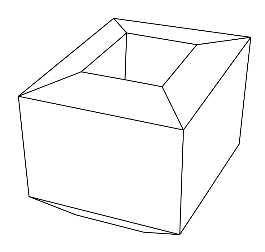
이로부터 우리는 $v - e + f$의 값이 도형의 위상에 의해 결정된다고 추측할 수 있다. 이것이 오일러-푸앵카레 정리의 내용이다. 정리를 진술하기 앞서, 먼저 다음의 개념을 정의하자.
정의. 위상공간 $X$에 대해, $X$의 호몰로지 군 $H_p(X)$의 자유 부분free part의 랭크를 $X$의 $p$번째 베티 수Betti number라고 하며 $R_p(X)$라고 적는다.
원래 $b_p(X)$라고 적는 것이 관행인데, 이 글에서는 $b_p$를 다른 의미로 사용할 것이기 때문에 다른 표기법을 채택했다. 호몰로지 군은 위상 불변이므로 베티 수 또한 위상 불변이다.
예를 들어 토러스의 호몰로지 군은 다음과 같다.
- $H_0(X) = \mathbb{Z}$
- $H_1(X) = \mathbb{Z} \oplus \mathbb{Z}$
- $H_2(X) = \mathbb{Z}$
따라서 토러스의 0차, 1차, 2차 베티 수는 각각 1, 2, 1이다. 베티 수는 직관적으로 구멍의 의미를 가진다 (이전 글 참조). 특히, 0차 베티 수는 $K$를 이루는 연결 요소들의 수이다. 즉, 두 개의 사면체를 하나의 단체 복합체로 간주한다면 이 복합체의 0차 베티 수는 2이다.
오일러-푸앵카레 정리. $n$-단체 복합체 $K$에 대해, $\alpha_p \; (p \leq n)$를 $K$의 $p$-단체들의 개수라고 하자. 다음이 성립한다.
\[\sum^n_{p = 0} (-1)^p\alpha_p = \sum^n_{p=0}(-1)^p R_p(K)\]
위 정리의 증명에서는 $p$-체인들을 자유군의 원소로 보는 것보다 선형 공간의 원소로 보는 것이 더 자연스럽기 때문에 이 접근을 취한다.
증명. $K$의 $p$-체인, 고리, 경계가 각각 유리수체에 대해 이루는 선형 공간을 $C_p, Z_p, B_p$라고 하자. $\lbrace d^i_p \rbrace $가 고리를 선형 생성하지 않는 $C_p$의 극대 부분집합이라고 하고, $\lbrace d^i_p \rbrace $가 생성하는 선형공간을 $D_p$라고 하자. 다음이 성립한다 ($\oplus$는 벡터 공간의 직합).
\[\begin{gather} C_p = D_p \oplus Z_p\\\\ \alpha_p = \dim C_p = \dim D_p + \dim Z_p \end{gather}\]$p \leq n - 1$에 대해, $b^i_p = \partial d^i_{p + 1}$라고 하자. $\lbrace b^i_p \rbrace $가 생성하는 선형 공간을 $B_p$라고 하자. $\partial$은 선형 연산자이므로, $\lbrace d^i_{p +1} \rbrace $가 $D_{p + 1}$의 선형 기저라는 사실로부터 $\lbrace b^i_p \rbrace $가 $B_p$의 선형 기저라는 사실이 따라 나온다. 다음의 보조정리를 증명한다.
보조정리. $B_p$는 $K$의 모든 $p$-경계들을 포함한다.
증명. 만약 $b_p$가 $K$의 $p$-경계라면, 어떤 $c_{p + 1} \in C_{p + 1}$에 대해 $\partial c_{p + 1} = b_p$이다. $C_{p + 1} = D_{p + 1} \oplus Z_{p + 1}$ 관계에 의해 어떤 유일한 $d_{p + 1} \in D_{p + 1}, z_{p + 1} \in Z_{p + 1}$이 존재하여 $c_{p + 1 } = d_{p + 1} + z_{p + 1}$이다. 그런데 $\partial z_{p + 1} = 0$이므로 $\partial d_{p + 1} = b_p$이다. 따라서 $b_p \in B_p$이다. □
$\lbrace z^i_p \rbrace $가 $B_p$의 원소를 선형 생성하지 않는 $Z_p$의 극대 부분집합이라고 하고, $\lbrace z^i_p \rbrace $가 생성하는 선형공간을 $G_p$라고 하자. 보조정리에 의해 다음이 성립한다.
\[\dim G_p = R_p\]따라서 다음이 성립한다.
\[\begin{gather} Z_p = B_p \oplus G_p\\\\ \dim Z_p = \dim B_p + \dim G_p = \dim D_{p + 1} + R_p \end{gather}\]앞선 결과와 연립하면 다음을 얻는다 ($p \leq n - 1$).
\[\alpha_p = \dim D_{p + 1} + \dim D_p + R_p\]$p = n$일 때 $\alpha_n = \dim D_n + R_n$이고, $p = 0$일 때 $\alpha_0 = \dim D_1 + R_0$이다. 따라서 다음을 얻는다 (wlog, $n$은 짝수).
\[\begin{alignat}{3} &\alpha_n &&= \;\cancel{\dim D_n} + R_p \\ &-\alpha_{n-1} &&= \;\cancel{-\dim D_{n}} \cancel{- \dim D_{n - 1}} - R_{n - 1} \\ &\alpha_{n-2} &&= \;\cancel{\dim D_{n - 1}} \cancel{ + \dim D_{n - 2}} + R_{n - 2} \\ &&\vdots \\ &-\alpha_{1} &&= \;\cancel{-\dim D_{2}} \cancel{-\dim D_{1}} - R_{1} \\ &\alpha_{0} &&= \;\cancel{\dim D_{1}} + R_{0} \\ \hline &\sum_{p = 0}^n (-1)^p \alpha_p &&= \;\sum_{p=0}^n (-1)^p R_p(K) \quad \blacksquare \end{alignat}\]정의. 위상공간 X에 대해, 다음 값을 오일러 종수Euler characteristic라고 한다.
\[\xi(X) = \sum (-1)^p R_p(X)\]
베티 수가 위상 불변이므로 오일러 종수 또한 위상 불변이다.
따름정리. 다면체 $P$의 꼭짓점, 모서리, 면의 개수를 $v, e, f$라고 하자. 2차원 위상공간으로서의 $P$의 표면을 $X$라고 하자. 다음이 성립한다.
\[v - e + f = \xi(X)\]
증명. $k$각형의 삼각화는 $k - 3$개의 모서리를 추가함으로써 얻을 수 있는데, 이 과정에서 $k - 3$개의 면이 생긴다. 따라서 $P$는 $P$의 삼각화와 $v - e + f$ 값이 같으며, 이는 오일러 종수와 같다. ■
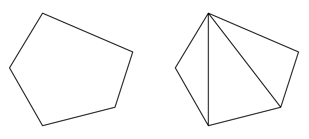
앞서 우리는 구멍이 하나 있는 다면체의 경우 $v - e + f = 0$임을 보았다. 실제로 토러스의 0차, 1차, 2차 베티 수는 1, 2, 1이며, $1 - 2 + 1 = 0$이다. 한편 구의 호몰로지 군은 다음과 같다.
- $H_0(K) = \mathbb{Z}$
- $H_1(K) = 0$
- $H_2(K) = \mathbb{Z}$
따라서 구의 0차, 1차, 2차 베티 수는 1, 0, 1이며, $1 - 0 + 1 = 2$이다. 따라서 볼록다면체의 경우 $v - e + f = 2$이다.
Euler-Poincaré Theorem
23 Nov 2025This post was originally written in Korean, and has been machine translated into English. It may contain minor errors or unnatural expressions. Proofreading will be done in the near future.
Readers may recall learning the following theorem in their youth:
Euler’s Formula. For a convex polyhedron, let $v, e, f$ denote the number of vertices, edges, and faces, respectively. Then $v - e + f = 2$.
For instance, in the case of a cube, $v = 8, e = 12, f = 6$, so $v - e + f = 2$ holds. The condition of convexity is crucial; if the polyhedron has “holes,” the formula does not hold. For example, in the case of the punctured prism below, $v = 16, e = 32, f = 16$, so $v - e + f = 0$.
From this, we may conjecture that the value of $v - e + f$ is determined by the topology of the shape. This is the essence of the Euler-Poincaré theorem. Before stating the theorem, let us first define the following concept:
Definition. For a topological space $X$, the rank of the free part of the homology group $H_p(X)$ of $X$ is called the $p$th Betti number of $X$, denoted $R_p(X)$.
While it is customary to denote this as $b_p(X)$, we adopt a different notation here as $b_p$ will be used for another purpose in this article. Since homology groups are topological invariants, Betti numbers are also topological invariants.
For example, the homology groups of a torus are as follows:
- $H_0(X) = \mathbb{Z}$
- $H_1(X) = \mathbb{Z} \oplus \mathbb{Z}$
- $H_2(X) = \mathbb{Z}$
Thus, the 0th, 1st, and 2nd Betti numbers of the torus are 1, 2, and 1, respectively. Intuitively, Betti numbers represent the number of “holes” (see previous post). In particular, the 0th Betti number corresponds to the number of connected components of $K$. For instance, if two tetrahedra are considered as a single simplicial complex, the 0th Betti number of this complex is 2.
Euler-Poincaré Theorem. For an $n$-dimensional simplicial complex $K$, let $\alpha_p \; (p \leq n)$ denote the number of $p$-simplices in $K$. Then the following holds:
\[\sum^n_{p = 0} (-1)^p\alpha_p = \sum^n_{p=0}(-1)^p R_p(K)\]
In proving this theorem, it is more natural to view $p$-chains as elements of a vector space rather than a free group, and we adopt this approach.
Proof. Let $C_p, Z_p, B_p$ denote the vector spaces of $p$-chains, cycles, and boundaries of $K$ over the field of rational numbers, respectively. Let $\lbrace d^i_p \rbrace $ be a maximal subset of $C_p$ that does not linearly generate cycles, and let the vector space spanned by $\lbrace d^i_p \rbrace $ be $D_p$. Then the following holds ($\oplus$ denotes the direct sum of vector spaces):
\[\begin{gather} C_p = D_p \oplus Z_p\\\\ \alpha_p = \dim C_p = \dim D_p + \dim Z_p \end{gather}\]For $p \leq n - 1$, let $b^i_p = \partial d^i_{p + 1}$. Let the vector space spanned by $\lbrace b^i_p \rbrace $ be $B_p$. Since $\partial$ is a linear operator, it follows from the fact that $\lbrace d^i_{p +1} \rbrace $ forms a basis of $D_{p + 1}$ that $\lbrace b^i_p \rbrace $ forms a basis of $B_p$. We prove the following lemma:
Lemma. $B_p$ contains all $p$-boundaries of $K$.
Proof. If $b_p$ is a $p$-boundary of $K$, then there exists some $c_{p + 1} \in C_{p + 1}$ such that $\partial c_{p + 1} = b_p$. By the relation $C_{p + 1} = D_{p + 1} \oplus Z_{p + 1}$, there exist unique $d_{p + 1} \in D_{p + 1}$ and $z_{p + 1} \in Z_{p + 1}$ such that $c_{p + 1 } = d_{p + 1} + z_{p + 1}$. Since $\partial z_{p + 1} = 0$, it follows that $\partial d_{p + 1} = b_p$. Hence, $b_p \in B_p$. □
Let $\lbrace z^i_p \rbrace $ be a maximal subset of $Z_p$ that does not linearly generate elements of $B_p$, and let the vector space spanned by $\lbrace z^i_p \rbrace $ be $G_p$. By the lemma, the following holds:
\[\dim G_p = R_p\]Thus, we have:
\[\begin{gather} Z_p = B_p \oplus G_p\\\\ \dim Z_p = \dim B_p + \dim G_p = \dim D_{p + 1} + R_p \end{gather}\]Combining this with earlier results, we obtain the following for $p \leq n - 1$:
\[\alpha_p = \dim D_{p + 1} + \dim D_p + R_p\]For $p = n$, $\alpha_n = \dim D_n + R_n$, and for $p = 0$, $\alpha_0 = \dim D_1 + R_0$. Hence, we derive the following (wlog, $n$ is even):
\[\begin{alignat}{3} &\alpha_n &&= \;\cancel{\dim D_n} + R_p \\ &-\alpha_{n-1} &&= \;\cancel{-\dim D_{n}} \cancel{- \dim D_{n - 1}} - R_{n - 1} \\ &\alpha_{n-2} &&= \;\cancel{\dim D_{n - 1}} \cancel{ + \dim D_{n - 2}} + R_{n - 2} \\ &&\vdots \\ &-\alpha_{1} &&= \;\cancel{-\dim D_{2}} \cancel{-\dim D_{1}} - R_{1} \\ &\alpha_{0} &&= \;\cancel{\dim D_{1}} + R_{0} \\ \hline &\sum_{p = 0}^n (-1)^p \alpha_p &&= \;\sum_{p=0}^n (-1)^p R_p(K) \quad \blacksquare \end{alignat}\]Definition. For a topological space $X$, the following value is called the Euler characteristic:
\[\xi(X) = \sum (-1)^p R_p(X)\]
Since Betti numbers are topological invariants, the Euler characteristic is also a topological invariant.
Corollary. Let $v, e, f$ denote the number of vertices, edges, and faces of a polyhedron $P$, respectively. Let $X$ denote the surface of $P$ as a 2-dimensional topological space. Then the following holds:
\[v - e + f = \xi(X)\]
Proof. The triangulation of a $k$-gon can be obtained by adding $k - 3$ edges, which creates $k - 3$ faces. Thus, $P$ has the same $v - e + f$ value as its triangulation, which equals the Euler characteristic. ■
Earlier, we observed that for a polyhedron with one hole, $v - e + f = 0$. Indeed, the 0th, 1st, and 2nd Betti numbers of a torus are 1, 2, and 1, respectively, and $1 - 2 + 1 = 0$. On the other hand, the homology groups of a sphere are as follows:
- $H_0(K) = \mathbb{Z}$
- $H_1(K) = 0$
- $H_2(K) = \mathbb{Z}$
Thus, the 0th, 1st, and 2nd Betti numbers of a sphere are 1, 0, and 1, respectively, and $1 - 0 + 1 = 2$. Therefore, for convex polyhedra, $v - e + f = 2$.
클럽 집합과 정상 집합
11 Nov 2025클럽 집합
정의. $C \subseteq \omega_1$이 클럽 집합club set이라는 것은 $C$가 닫히고 무계closed and unbounded라는 것이다. 즉,
- 임의의 서수열 $(\alpha_n)_{n \in \omega} \subseteq C$에 대해 $\alpha_n \to \alpha$라면 $\alpha \in C$이다.
- 임의의 $\gamma < \kappa$에 대해 $\alpha > \gamma$인 $\alpha \in C$가 존재한다.
그야말로 정직한 네이밍이 아닐 수 없다.
정리. $C_1, C_2 \subseteq \omega_1$이 두 클럽 집합일 때, $C = C_1 \cap C_2$ 또한 클럽 집합이다.
증명. $C$가 닫힘이라는 것은 쉽게 보여진다. $C$가 무계임을 보이기 위해 임의의 $\gamma \in \omega_1$를 잡자. $C_1$이 무계이므로 $\gamma < \alpha_0$을 만족하는 가장 작은 $\alpha_0 \in C_1$가 있다. $C_2$가 무계이므로 $\alpha_0 < \beta_0$인 가장 작은 $\beta_0 \in C_2$가 있다. 다시 $C_1$이 무계이므로 $\beta_0 < \alpha_1$인 $\alpha_1 \in C_1$가 있다. 이 과정을 계속 반복하여 서수열 $\lbrace \alpha_n \rbrace $과 $\lbrace \beta_n \rbrace $을 얻는다. 두 서수열은 같은 서수 $\delta$로 수렴하므로 $\delta \in C$이며, $\delta > \gamma$이다. (p.s. “가장 작은”은 불필요한 선택 공리의 사용을 피하기 위해 사용되었다) ■
위 증명을 살짝 변형하면 다음 정리를 얻을 수 있다.
정리. $\lbrace C_n \rbrace _{n < \omega}$가 클럽 집합들의 가산 모임일 때, $C = \bigcap C_n$ 또한 클럽 집합이다.
증명. 연습문제 (힌트: 삼각형을 사용한다) ■
따라서 가산 개의 클럽 집합들이 주어지면 교집합을 취함으로써 새로운 클럽 집합을 얻을 수 있다. 한편, 비가산 개의 클럽 집합들이 주어지면 다음을 사용할 수 있다.
정리. $\lbrace C_\xi \rbrace _{\xi < \omega_1}$이 클럽 집합들의 모임일 때, $\lbrace C_\xi \rbrace $의 대각 교집합diagonal intersection을 다음과 같이 정의한다.
\[\Delta_{\xi < \omega_1} C_\xi = \{ \alpha \in \omega_1 : \forall \xi < \alpha \;\; \alpha \in C_\xi \}\]$D$는 클럽 집합이다.
증명. $D$가 닫혀 있음을 먼저 보이자. 서수열 $(\alpha_n)_{n \in \omega} \subseteq D$에 대해 $\alpha_n \to \alpha$라고 하자. 임의의 $\xi < \alpha$에 대해 $\xi < \alpha_n$인 $n \in \omega$가 존재하며, 대각 교집합의 정의에 의해 $C_\xi$은 $\lbrace \alpha_m : m \geq n \rbrace $을 포함한다. 따라서 $\sup \lbrace \alpha_m : m \geq n \rbrace = \alpha \in C_\xi$이므로 $\alpha \in D$이다.
이제 $D$가 무계임을 보이자. 임의의 $\gamma < \omega_1$에 대해, $D_0 = \bigcap_{\xi < \gamma} C_\xi$는 클럽 집합이므로 무계이다. 따라서 $\alpha_0 > \gamma$를 만족하는 가장 작은 $\alpha_0 \in D_0$가 존재한다. 마찬가지로 $D_1 = \bigcap_{\xi < \alpha_0} C_\xi$가 클럽 집합이므로 $\alpha_1 > \alpha_0$를 만족하는 가장 작은 $\alpha_1 \in D_1$이 존재한다. 이 과정을 귀납적으로 반복하여 얻은 서수열 $(\alpha_n)$의 극한이 $\alpha$라고 하자. 임의의 $\xi < \alpha$에 대해, 어떤 $n$이 존재하여 $\xi < \alpha_n$이므로 임의의 $m \geq n$에 대하여 $\alpha_m \in C_\xi$이다. 따라서 $\alpha \in C_\xi$이며 $\alpha \in D$이다. ■
$\Delta C_\xi \supseteq \bigcap C_\xi$임을 확인하라.
참고로 지금까지의 정의와 정리들은 다음과 같이 일반화될 수 있다. $\kappa$가 $\operatorname{cf}\kappa > \omega$인 비가산 기수라고 하자.
정의. $C \subseteq \kappa$가 클럽 집합club set이라는 것은 $C$가 닫히고 무계closed and unbounded라는 것이다. 즉,
- 임의의 $\alpha < \kappa$에 대해 $\sup (C \cap \alpha) = \alpha$라면 (즉 $C$가 $\alpha$에서 무계라면) $\alpha \in C$이다.
- 임의의 $\gamma < \kappa$에 대해 $\alpha > \gamma$인 $\alpha \in C$가 존재한다.
정리. $\lambda < \operatorname{cf}\kappa$에 대해 $\lbrace C_\xi \rbrace _{\xi < \lambda}$가 클럽 집합들의 모임일 때, $C = \bigcap C_\xi$ 또한 클럽 집합이다.
정리. $\kappa$가 정칙regular이라면, $\lbrace C_\xi \rbrace _{\xi < \kappa}$가 클럽 집합들의 모임일 때, $\lbrace C_\xi \rbrace $의 대각 교집합 또한 클럽 집합이다.
증명. $\kappa = \omega_1$인 경우와 거의 같다. ■
정상 집합
유한 교집합 닫힘에 의해 클럽 집합들의 모임은 필터를 생성한다. 해당 필터의 쌍대dual 아이디얼에 속하지 않는 집합을 정상 집합stationary set이라고 한다. 다른 말로 하자면 다음과 같다.
정의. $S \subseteq \omega_1$이라고 하자. 임의의 클럽 집합 $C \subseteq \omega_1$에 대해 $C \cap S \neq \varnothing$이라면 $S$는 정상 집합이다.
어떤 클럽 집합 $C$에 대해 $C \cap S = \varnothing$이라면 $S^c \subseteq C$이므로 $C$는 쌍대 아이디얼의 원소이다. 따라서 두 정의는 동치이다.
정상 집합은 $\omega_1$의 부분집합 중 “유의미하게 큰” 집합들을 포착한다. 이 사실은 다음의 (엄밀하지는 않은) 유비를 통해 더 잘 이해할 수 있다. $\omega_1$의 측도가 1이라고 할 때, 클럽 집합은 $\mu(C) = 1$인 집합에, 정상 집합은 $\mu(S) > 0$인 집합에 대응된다.
다음의 사실들은 쉽게 증명될 수 있다 (1번과 3번이 측도 유비와 자연스럽게 연결되는 것에 주목하라).
정리. 다음이 성립한다.
- 모든 클럽 집합은 정상 집합이다.
- 모든 정상 집합은 무계이다.
- $\bigcup_{n < \omega} A_n$가 정상 집합이라면 어떤 $m \in \omega$에 대해 $A_m$은 정상 집합이다.
정상 집합의 이름이 stationary인 이유는 다음의 정리 때문이다.
정리. $S \subseteq \omega_1$에 대해, $f: S \to \omega_1$이 퇴행적regressive이라는 것은 임의의 $\alpha \in S$에 대해 $f(\alpha) < \alpha$라는 것이다. 다음이 동치이다.
- $S$는 정상 집합이다.
- 임의의 퇴행적 함수 $f: S \to \omega_1$에 대해, $f$는 어떤 무계 집합 $T \subseteq S$ 위에서 상수constant이다.
- 임의의 퇴행적 함수 $f: S \to \omega_1$에 대해, $f$는 어떤 정상 집합 $T \subseteq S$ 위에서 상수이다.
증명. 3 ⇒ 2는 자명하므로, 1 ⇒ 3과 2 ⇒ 1을 증명하면 된다.
1 ⇒ 3
대우를 증명한다. 어떤 퇴행적 함수 $f: S \to \omega_1$에 대해, $S$의 모든 정상 부분집합 위에서 $f$가 상수가 아니라고 하자. 즉, 임의의 $\xi \in \omega_1$에 대하여 $A_\xi = f^{-1}(\lbrace \xi \rbrace )$는 정상 집합이 아니다. 따라서 $A_\xi \cap C_\xi = \varnothing$인 클럽 집합 $C_\xi$가 존재한다.
$D = \Delta_{\xi < \omega_1} C_\xi$라고 하자. $D$는 클럽 집합이므로, 만약 $S$가 정상 집합이라면 $D \cap S \neq \varnothing$이다. $\alpha \in D \cap S$라고 하자. $\alpha \in D$이므로 임의의 $\xi < \alpha$에 대하여 $\alpha \in C_\xi$이다. 즉, $\alpha \notin A_\xi$이므로 $f(\alpha) \neq \xi$이다. 그런데 $\alpha \in S$이므로 $f(\alpha) < \alpha$이다. 이는 모순이므로 $S$는 정상 집합이 아니다. □
2 ⇒ 1
마찬가지로 대우를 증명한다. $S$가 정상 집합이 아니라고 하자. 그러면 어떤 클럽 집합 $C$에 대해 $S \cap C = \varnothing$이다. 다음의 함수를 정의하자.
\[f(\alpha) = \sup (C \cap \alpha)\]임의의 $\alpha \in S$에 대하여 $f(\alpha) \leq \alpha$이다. 만약 $f(\alpha) = \alpha$라면, $C$는 $\alpha$로 수렴하는 서수열을 가진다. 그런데 $C$는 닫힌 집합이므로, $\alpha \in C$이다. 이는 $S \cap C = \varnothing$에 모순이다. 따라서 $f(\alpha) < \alpha$이며, $f$는 퇴행적이다.
만약 어떤 무계 집합 $T$ 위에서 $f$의 값이 $\gamma < \omega_1$로 일정했다면, 어떤 무계인 서수열 $(\alpha_n)$에 대해 $\sup (C \cap \alpha_n) = \gamma$이다. 그런데 $C$는 무계이므로, 이는 $\sup \alpha_n = \gamma$를 함축한다. 그런데 $(\alpha_n)$이 무계이므로 $\sup \alpha_n = \omega_1$이다. 이는 모순이다. 따라서 $f$는 어떠한 무계 집합 위에서도 상수가 아닌 퇴행적 함수이다. ■
위 정리는 다음의 정리로 일반화될 수 있다.
포더 보조정리Fodor’s lemma. $\kappa$가 비가산 정칙 기수라고 하자. 임의의 $S \subseteq \kappa$에 대해 다음이 동치이다.
- $S$는 정상 집합이다.
- 임의의 퇴행적 함수 $f: S \to \omega_1$에 대해, $f$는 어떤 무계 집합 $T \subseteq S$ 위에서 상수이다.
- 임의의 퇴행적 함수 $f: S \to \omega_1$에 대해, $f$는 어떤 정상 집합 $T \subseteq S$ 위에서 상수이다.
정상 집합의 응용
정상 집합의 한 응용으로서 조합론의 다음 정리를 보자.
Δ-계 보조정리Δ-system lemma. $\lbrace A_\xi\rbrace _{\xi < \omega_1}$가 $\omega_1$의 유한부분집합들의 모임이라고 하자. 어떤 무계인 $I \subseteq \omega_1$와 유한집합 $A$가 존재하여, 임의의 $i, j \in I, i \neq j$에 대해 $A_i \cap A_j = A$이다.
증명. 비둘기집의 원리에 의해 일반성을 잃지 않고, 임의의 $\xi < \omega_1$에 대해 $|A_\xi | = n$이라고 가정할 수 있다. 다음과 같이 정의하자.
\[C = \{ \alpha < \omega_1 : \forall \xi < \alpha \;\; \operatorname{max}C_\xi < \alpha \}\]$C$는 클럽 집합이다. 또한 $0 \leq k \leq n$에 대해 다음과 같이 정의하자.
\[T_k = \{ \alpha \in C : |A_\alpha \cap \alpha | = k \}\]$\bigcup_{0 \leq k \leq n} T_k = C$이므로 어떤 $m$에 대해 $T_m$은 정적 집합이다. 이제 $0 \leq l < m$에 대해 다음의 함수를 정의하자.
\[f_l(\alpha) : T_m \to \omega_1; \quad \alpha \mapsto \text{$l$th element of $A_\alpha$}\]$|A_\alpha \cap \alpha| > l$이므로 $f_l(\alpha) < \alpha$이다. 따라서 각 $l$에 대해 $f_l$는 퇴행적이다. 이제 다음의 단계를 반복한다.
- $f_0$가 상수가 되는 정적 집합 $S_0 \subseteq T_m$이 존재한다.
- $f_1 |_{S_0}$이 상수가 되는 정적 집합 $S_1 \subseteq S_0$가 존재한다.
- $f_2 |_{S_1}$이 상수가 되는 정적 집합 $S_2 \subseteq S_1$이 존재한다.
- …
- $f_{m-1} |_{S_{m-2}}$가 상수가 되는 정적 집합 $S_{m-1} \subseteq S_{m-2}$가 존재한다.
그러면 임의의 $0 \leq l < m$에 대해 $f_l$은 $S_{m-1}$에서 상수이다. 이제 $S_{m-1} = I$가 찾고자 하는 집합임을 쉽게 확인할 수 있다. ■
Club Sets and Stationary Sets
11 Nov 2025This post was originally written in Korean, and has been machine translated into English. It may contain minor errors or unnatural expressions. Proofreading will be done in the near future.
Club Sets
Definition. $C \subseteq \omega_1$ is a club set if $C$ is closed and unbounded. That is,
- For any sequence of ordinals $(\alpha_n)_{n \in \omega} \subseteq C$, if $\alpha_n \to \alpha$, then $\alpha \in C$.
- For any $\gamma < \kappa$, there exists $\alpha \in C$ such that $\alpha > \gamma$.
The name is indeed quite straightforward.
Theorem. If $C_1, C_2 \subseteq \omega_1$ are two club sets, then $C = C_1 \cap C_2$ is also a club set.
Proof. It is easy to show that $C$ is closed. To prove that $C$ is unbounded, let us take an arbitrary $\gamma \in \omega_1$. Since $C_1$ is unbounded, there exists the smallest $\alpha_0 \in C_1$ such that $\gamma < \alpha_0$. Similarly, since $C_2$ is unbounded, there exists the smallest $\beta_0 \in C_2$ such that $\alpha_0 < \beta_0$. Again, since $C_1$ is unbounded, there exists $\alpha_1 \in C_1$ such that $\beta_0 < \alpha_1$. Repeating this process, we obtain sequences of ordinals $\lbrace \alpha_n \rbrace$ and $\lbrace \beta_n \rbrace$. These sequences converge to the same ordinal $\delta$, so $\delta \in C$ and $\delta > \gamma$. (Note: “the smallest” is used to avoid unnecessary reliance on the axiom of choice.) ■
By slightly modifying the above proof, we can derive the following theorem.
Theorem. If $\lbrace C_n \rbrace _{n < \omega}$ is a countable collection of club sets, then $C = \bigcap C_n$ is also a club set.
Proof. Exercise (Hint: Use a triangle argument). ■
Thus, given a countable collection of club sets, we can obtain a new club set by taking their intersection. On the other hand, if we are given an uncountable collection of club sets, the following result can be used.
Theorem. Let $\lbrace C_\xi \rbrace _{\xi < \omega_1}$ be a collection of club sets. The diagonal intersection of $\lbrace C_\xi \rbrace$ is defined as follows:
\[\Delta_{\xi < \omega_1} C_\xi = \{ \alpha \in \omega_1 : \forall \xi < \alpha \;\; \alpha \in C_\xi \}\]$D$ is a club set.
Proof. First, let us show that $D$ is closed. Suppose $(\alpha_n)_{n \in \omega} \subseteq D$ and $\alpha_n \to \alpha$. For any $\xi < \alpha$, there exists $n \in \omega$ such that $\xi < \alpha_n$. By the definition of the diagonal intersection, $C_\xi$ contains $\lbrace \alpha_m : m \geq n \rbrace$. Hence, $\sup \lbrace \alpha_m : m \geq n \rbrace = \alpha \in C_\xi$, so $\alpha \in D$.
Next, let us show that $D$ is unbounded. For any $\gamma < \omega_1$, let $D_0 = \bigcap_{\xi < \gamma} C_\xi$. Since $D_0$ is a club set, it is unbounded. Thus, there exists the smallest $\alpha_0 \in D_0$ such that $\alpha_0 > \gamma$. Similarly, let $D_1 = \bigcap_{\xi < \alpha_0} C_\xi$. Since $D_1$ is a club set, there exists the smallest $\alpha_1 \in D_1$ such that $\alpha_1 > \alpha_0$. Repeating this process inductively, we obtain a sequence $(\alpha_n)$ whose limit is $\alpha$. For any $\xi < \alpha$, there exists $n$ such that $\xi < \alpha_n$, and for all $m \geq n$, $\alpha_m \in C_\xi$. Hence, $\alpha \in C_\xi$ and $\alpha \in D$. ■
Verify that $\Delta C_\xi \supseteq \bigcap C_\xi$.
The definitions and theorems discussed so far can be generalised as follows. Let $\kappa$ be an uncountable cardinal with $\operatorname{cf}\kappa > \omega$.
Definition. $C \subseteq \kappa$ is a club set if $C$ is closed and unbounded. That is,
- For any $\alpha < \kappa$, if $\sup (C \cap \alpha) = \alpha$ (i.e., $C$ is unbounded at $\alpha$), then $\alpha \in C$.
- For any $\gamma < \kappa$, there exists $\alpha \in C$ such that $\alpha > \gamma$.
Theorem. If $\lambda < \operatorname{cf}\kappa$ and $\lbrace C_\xi \rbrace _{\xi < \lambda}$ is a collection of club sets, then $C = \bigcap C_\xi$ is also a club set.
Theorem. If $\kappa$ is regular, then the diagonal intersection of a collection $\lbrace C_\xi \rbrace _{\xi < \kappa}$ of club sets is also a club set.
Proof. The proof is almost identical to the case $\kappa = \omega_1$. ■
Stationary Sets
By closure under finite intersections, the collection of club sets generates a filter. A set that does not belong to the dual ideal of this filter is called a stationary set. In other words:
Definition. Let $S \subseteq \omega_1$. If $C \cap S \neq \varnothing$ for every club set $C \subseteq \omega_1$, then $S$ is a stationary set.
If there exists a club set $C$ such that $C \cap S = \varnothing$, then $S^c \subseteq C$, so $C$ belongs to the dual ideal. Thus, the two definitions are equivalent.
Stationary sets capture “significantly large” subsets of $\omega_1$. This can be better understood through the following (informal) analogy: if $\omega_1$ has measure 1, then club sets correspond to sets with $\mu(C) = 1$, and stationary sets correspond to sets with $\mu(S) > 0$.
The following facts are easily proven (note how 1 and 3 naturally align with the measure analogy):
Theorem. The following hold:
- Every club set is a stationary set.
- Every stationary set is unbounded.
- If $\bigcup_{n < \omega} A_n$ is a stationary set, then there exists some $m \in \omega$ such that $A_m$ is a stationary set.
The name “stationary” for stationary sets arises from the following theorem.
Theorem. Let $S \subseteq \omega_1$. A function $f: S \to \omega_1$ is regressive if $f(\alpha) < \alpha$ for all $\alpha \in S$. The following are equivalent:
- $S$ is a stationary set.
- For any regressive function $f: S \to \omega_1$, $f$ is constant on some unbounded set $T \subseteq S$.
- For any regressive function $f: S \to \omega_1$, $f$ is constant on some stationary set $T \subseteq S$.
Proof. 3 ⇒ 2 is trivial, so it suffices to prove 1 ⇒ 3 and 2 ⇒ 1.
1 ⇒ 3
We prove the contrapositive. Suppose there exists a regressive function $f: S \to \omega_1$ such that $f$ is not constant on any stationary subset of $S$. That is, for every $\xi \in \omega_1$, $A_\xi = f^{-1}(\lbrace \xi \rbrace)$ is not stationary. Hence, there exists a club set $C_\xi$ such that $A_\xi \cap C_\xi = \varnothing$.
Let $D = \Delta_{\xi < \omega_1} C_\xi$. Since $D$ is a club set, if $S$ is stationary, then $D \cap S \neq \varnothing$. Let $\alpha \in D \cap S$. Since $\alpha \in D$, for any $\xi < \alpha$, $\alpha \in C_\xi$. Thus, $\alpha \notin A_\xi$, so $f(\alpha) \neq \xi$. However, since $\alpha \in S$, $f(\alpha) < \alpha$. This is a contradiction, so $S$ is not stationary. □
2 ⇒ 1
We again prove the contrapositive. Suppose $S$ is not stationary. Then there exists a club set $C$ such that $S \cap C = \varnothing$. Define the following function:
\[f(\alpha) = \sup (C \cap \alpha)\]For any $\alpha \in S$, $f(\alpha) \leq \alpha$. If $f(\alpha) = \alpha$, then $C$ contains a sequence of ordinals converging to $\alpha$. Since $C$ is closed, $\alpha \in C$. This contradicts $S \cap C = \varnothing$. Thus, $f(\alpha) < \alpha$, and $f$ is regressive.
If $f$ were constant on some unbounded set $T$, then for some $\gamma < \omega_1$, there would exist an unbounded sequence $(\alpha_n)$ such that $\sup (C \cap \alpha_n) = \gamma$. Since $C$ is unbounded, this implies $\sup \alpha_n = \gamma$. However, since $(\alpha_n)$ is unbounded, $\sup \alpha_n = \omega_1$. This is a contradiction. Thus, $f$ is a regressive function that is not constant on any unbounded set. ■
The above theorem can be generalised as follows:
Fodor’s Lemma. Let $\kappa$ be an uncountable regular cardinal. For any $S \subseteq \kappa$, the following are equivalent:
- $S$ is a stationary set.
- For any regressive function $f: S \to \omega_1$, $f$ is constant on some unbounded set $T \subseteq S$.
- For any regressive function $f: S \to \omega_1$, $f$ is constant on some stationary set $T \subseteq S$.
Applications of Stationary Sets
As an application of stationary sets, consider the following combinatorial theorem:
Δ-System Lemma. Let $\lbrace A_\xi\rbrace _{\xi < \omega_1}$ be a collection of finite subsets of $\omega_1$. There exist an unbounded set $I \subseteq \omega_1$ and a finite set $A$ such that for any $i, j \in I$ with $i \neq j$, $A_i \cap A_j = A$.
Proof. By the pigeonhole principle, we may assume without loss of generality that $|A_\xi | = n$ for all $\xi < \omega_1$. Define:
\[C = \{ \alpha < \omega_1 : \forall \xi < \alpha \;\; \operatorname{max}C_\xi < \alpha \}\]$C$ is a club set. For $0 \leq k \leq n$, define:
\[T_k = \{ \alpha \in C : |A_\alpha \cap \alpha | = k \}\]Since $\bigcup_{0 \leq k \leq n} T_k = C$, there exists some $m$ such that $T_m$ is stationary. For $0 \leq l < m$, define:
\[f_l(\alpha) : T_m \to \omega_1; \quad \alpha \mapsto \text{$l$th element of $A_\alpha$}\]Since $|A_\alpha \cap \alpha| > l$, $f_l(\alpha) < \alpha$. Thus, $f_l$ is regressive. Now, repeat the following steps:
- There exists a stationary set $S_0 \subseteq T_m$ such that $f_0$ is constant on $S_0$.
- There exists a stationary set $S_1 \subseteq S_0$ such that $f_1 |_{S_0}$ is constant on $S_1$.
- There exists a stationary set $S_2 \subseteq S_1$ such that $f_2 |_{S_1}$ is constant on $S_2$.
- …
- There exists a stationary set $S_{m-1} \subseteq S_{m-2}$ such that $f_{m-1} |_{S_{m-2}}$ is constant on $S_{m-1}$.
For each $0 \leq l < m$, $f_l$ is constant on $S_{m-1}$. It is now easy to verify that $S_{m-1} = I$ is the desired set. ■
수학과 윤리학은 같은 배를 탔는가? 진화론 논변을 중심으로
07 Nov 2025이 글은 Justin Clarke-Doane, Morality and Mathematics: The Evolutionary Challenge (2012)를 정리한 것이다. “저자”는 논문의 저자를, “필자”는 이 글의 필자를 가리킨다. “도덕”과 “윤리”의 혼용을 방지하기 위해 “윤리”로 표현을 통일했다.
개요
윤리 실재론에 대한 반론 중 하나는 진화론 논변The Evolutionary Challenge이다. 진화론 논변에 따르면, 오늘날의 인류가 가지는 윤리적 믿음들은 진화적 압력evolutionary forces에 의해 형성되었다. 그러나 진화의 원리는 윤리적 사실들과 무관하므로, 윤리적 사실들이 완전히 다른 반사실적 세계에서도 인류는 동일한 윤리적 믿음들을 가지도록 진화했을 것이다. 그러므로 만약 우리의 윤리적 믿음들이 참이라면 이는 진화의 결과와 윤리의 명제들이 굉장한 우연으로 일치하게 된 것이다. 따라서 진화론 논변을 옹호하는 자들은 윤리 실재론이 굉장한 우연을 날것 그대로 받아들이거나, 혹은 우리의 윤리적 믿음들이 참이라고 생각할 근거가 없음을 인정해야 한다고 주장한다.
예를 들어 우리가 “타인을 배려해야 한다”라는 윤리적 믿음을 가지게 된 이유는, 아마 인류의 진화에 있어 상호 협력을 중시하는 집단이 이기주의를 중시하는 집단보다 생존 확률이 높았기 때문일 것이다. 그런데 상호 협력이 이기주의보다 생존 확률이 높다는 것은 윤리적 사실이 아니라, 두 전략의 기댓값에 대한 게임이론적 내지는 수학적 사실이다. 따라서 설령 상호 협력보다 이기주의가 윤리적이었다고 하더라도, 우리는 “타인을 배려해야 한다”라는 믿음을 가지도록 진화했을 것이다.
한편으로 진화론 논변은 수학 실재론을 위협하지는 않는 것으로 받아들여져 왔다. 왜냐하면 진화의 원리는 수학적 참에 의존적인 것으로 보이기 때문이다. 예를 들어 1 + 1 = 2임을 믿는 개체들은 그렇지 않은 개체보다 생존에 유리한데, 이는 1 + 1 = 2가 실제로 참이기 때문이다. 이를 조이스는 다음과 같이 설명한다.
수풀 A 뒤에 사자 한 마리가 있고 수풀 B 뒤에 사자 한 마리가 있다고 하자. 우리의 선조 P와 Q가 수풀 C 뒤에 숨어 있다. P는 사자 한 마리와 다른 사자 한 마리는 총 사자 두 마리가 된다고 믿고, Q는 사자 한 마리와 다른 사자 한 마리가 총 사자 0마리가 된다고 믿는다. 그렇다면 P가 Q보다 죽을 확률이 적으며, 자신의 유전자를 남길 확률이 크다. 왜냐하면 P는 Q보다 수풀 C에서 걸어나와 두 마리의 사자에게 잡아먹힐 확률이 적기 때문이다. 그러나 이 사실[이탤릭체로 표시된 사실]에 대한 설명은, 사자 한 마리와 다른 사자 한 마리가 정말로 0마리가 아니라 두 마리의 사자라는 사실을 전제한다.
그러나 논문에서 저자는 이것이 잘못된 생각이라고 주장한다. 저자는 진화론 논변이 윤리 실재론을 위협하는 것과 같은 정도로 수학 실재론을 위협한다고 주장한다. 결론적으로 저자는 윤리 실재론과 수학 실재론 중 하나만 받아들이는 입장은 비정합적이라고 피력한다.
1. 실재론은 정확히 무엇인가?
본 논증에 들어가기 앞서 저자는 윤리 실재론과 수학 실재론이 정확히 무엇을 의미하는지를 해명하고자 한다. 일반적으로, 저자는 어떤 논의 영역area of discourse D에 대해, D-실재론을 다음 네 입장의 연언으로 정의한다.
- D-참-적합성D-Truth-Aptness. D의 문장들은 진릿값을 가진다.
- D-참D-Truth. 어떤 D의 원자명제 또는 존재 양화 명제는 참이다.
- D-독립성D-Independence. D의 문장들의 진릿값은 정신과 언어에 유의미한 의미에서 독립적이다.
- D-액면성D-Literalness. D의 문장들은 문자 그대로 받아들여져야 한다.
D를 윤리학으로 설정할 경우 1은 에이어의 감정주의emotivism1를 기각하고, 2는 매키의 오류 이론error theory2을 기각하고, 3은 구성주의constructivism3를 기각하고, 4는 하먼의 상대주의4를 기각한다. D를 수학으로 설정할 경우 1은 힐베르트의 형식주의formalism5를 기각하고, 2는 필드의 허구주의fictionalism6를 기각하고, 3은 브라우어르 구성주의7를 기각하고, 4는 만약주의if-thenism8를 기각한다.
이 논문에서는 윤리 실재론과 수학 실재론을 기본적으로 전제한 뒤, 이들이 진화론 논변을 극복할 수 있는지 검토한다. 추가로 우리의 윤리적, 수학적 믿음들은 대부분 참이라고 전제한다.
2. 윤리 실재론에 대한 진화론 논변
실재론의 구성 요건을 밝혔으니, 진화론 논변이 어떻게 윤리 실재론을 공격하는지 살펴보자. 진화론 논변의 전제는 다음과 같다.
강한 전제. 우리의 윤리적 믿음은 참-독립적인 진화적 압력에 의해 형성되었다.
강한 전제는 다음 두 전제로 이루어져 있다.
E. 우리의 윤리적 믿음은 진화적으로 형성되었다.
NTT. 윤리적 믿음의 진화는 참-독립적non-truth-tracking으로 이루어졌다.
NTT의 정확한 의미는 다음의 반사실적 조건문이다.
P. 나머지 사실은 모두 유지된 채 오직 윤리적 사실만이 현실과 아주 달랐다고 하자. 그럼에도 우리는 현실에서 참인 윤리적 믿음들을 가지도록 진화했을 것이다.
혹자는 P 대신 Q를 2의 의미로 해명할 수 있다고 지적할 수 있다.
Q. 우리는 틀린 윤리적 믿음들을 가지도록 진화할 수 있었다.
그러나 저자는 Q가 견지될 수 없는 입장이라고 주장한다. 물론, 다윈이 일찍이 지적했듯이 인류가 꿀벌과 같은 환경에서 발생했다면 인류는 결혼하지 않은 여성이 형제를 죽이는 것을 용인했을지 모른다. 그러나 이 사례 자체는 Q를 예증하지 않는다. 해당 사례가 Q를 예증하기 위해서는 “꿀벌과 같은 환경에서 결혼하지 않은 여성이 형제를 죽이는 것은 잘못되었다”가 윤리적 참이라는 추가적인 가정이 필요한데, 이는 자명한 가정이 아니기 때문이다. (기아가 빈번했던 전근대 사회에서의 영아 살해와 현대의 영아 살해가 가지는 윤리적 무게를 고려해 보라.) 따라서 저자는 Q를 예증하고자 할 경우 “고통은 좋다”, “쾌는 나쁘다”와 같이 기초적explanatorily basic으로 틀린 윤리적 믿음들을 가지게 되는 경우를 제시해야 한다고 주장한다. 그러나 고통이 좋고 쾌가 나쁘다고 믿는 개체들은 진화론적으로 절멸했을 것이므로 Q는 견지될 수 없다. 따라서 P가 NPP의 올바른 해명이다.
그러나 P에도 문제가 있다. 많은 윤리 실재론자들은 윤리적 속성과 기술적descriptive 속성의 동일시가 형이상학적으로 필연적metaphysically necessary이라고 주장한다. 예를 들어 “쾌는 좋다”가 참이라면, 이 참은 형이상학적으로 필연적이다. 이 관점에 따르면 기술적 사실들이 고정된 채 윤리적 사실들만 달라지는 것은 형이상학적으로 불가능하다. 따라서 P에 대한 다음의 독해는 견지될 수 없다.
P1. 형이상학적인 의미에서 나머지 사실은 모두 유지된 채 오직 윤리적 사실만이 현실과 아주 달랐다고 하자. 그럼에도 우리는 현실에서 참인 윤리적 믿음들을 가지도록 진화했을 것이다.
대신 저자는 P를 다음과 같이 이해해야 한다고 주장한다.
P2. 나머지 사실은 모두 유지된 채 오직 윤리적 사실만이 현실과 아주 다른 상황을 정합적으로 상상해 보자intelligibly imagine. 그럼에도 우리는 현실에서 참인 윤리적 믿음들을 가지도록 진화했을 것이다.
수학을 예시로 들어, $\zeta(-1)$을 구하는 문제의 답을 $-1/12$로 찍어서 맞힌 아이의 경우를 생각해 보자. $\zeta(-1) = -1/12$은 필연적이므로, “이 문제의 답이 달랐더라도 아이는 정답을 맞혔을 것이다 (아이의 대답은 참-의존적truth-tracking이었다)”라는 반사실적 가정문은 형이상학적으로 공허참이다. 그럼에도 우리는 $\zeta(-1) = -1/12$이 아닌 경우를 상상할 수 있으며, 이 상상을 정합적으로intelligibly 전개한다면 아이는 문제를 틀렸을 것이다. 이런 의미에서 아이의 대답은 참-독립적이었다.
E와 NTT의 의미가 해명되었으므로, 강한 전제로부터 어떻게 윤리 실재론에 대한 반박을 유도하는지 살펴보자. 스트리트 등은 다음의 논변을 제시한다.
- 윤리적 사실이 아주 달라지는 것이 형이상학적으로는 불가능하더라도 그런 경우를 상상할 수는 있다.
- 우리가 상상할 수 있는 한에서, 윤리적 사실이 아주 달랐더라도 우리가 진화론적으로 형성하게 된 윤리적 믿음들은 동일했을 것이다.
- 따라서 현실의 우리가 윤리적으로 참인 믿음들을 가지게 되었다는 것은 설명될 수 없는 우연이다.
그러나 저자는 2로부터 3이 따라 나오지는 않는다고 주장한다. 2로부터 3을 도출하기 위해서는 다음의 일반적인 원리를 전제해야 한다.
D에 대한 기본적인 사실들이 달라지더라도 D에 대한 믿음들 중 달라지지 않는 믿음들의 참은 우연적이다.
저자는 위 원리에 대한 다음 반례를 든다. 철수는 자신을 향해 날아오는 농구공을 보며, “농구공이 내 눈앞으로 날라오고 있다”라고 믿는다. 여기서 농구공이 농구공처럼 배열된 원자들atoms arranged basketballwise과 같다는 것은 형이상학적으로 필연적이다. 그러나 우리는 물질이 원자가 아닌 다른 요소로 구성된 세계를 상상할 수 있다. 그런 세계에 사는 철수 앞으로 농구공이 날라오더라도 철수는 동일한 믿음, 즉 “농구공이 내 눈앞으로 날라오고 있다”라고 믿을 것이다. 이처럼 농구공에 대한 기본적인 사실들이 달라지더라도 철수는 동일한 믿음을 견지하지만, 그럼에도 불구하고 현실의 철수가 “농구공이 내 앞으로 날라오고 있다”라고 믿는 것은 참이며, 이 참은 우연적이지 않다.
필자 주: 필자는 저자가 잘못된 유비를 들었다고 생각한다. 농구공이 원자로 구성된 세계의 철수가 “농구공이 내 앞으로 날라오고 있다”라고 믿는 것과, 농구공이 연속체로 구성된 세계의 철수가 “농구공이 내 앞으로 날라오고 있다”라고 믿는 것은 동일한 믿음이 아니다. 왜냐하면 두 철수에게 있어 “농구공”의 의미는 지시ostension를 통해 결정되기 때문이다. 따라서 전자의 철수는 “농구공”으로 “농구공처럼 배열된 원자들”을 의미하고, 후자의 철수는 “농구공”으로 “농구공처럼 응축된 연속체”를 의미한다. 이렇듯 농구공에 대한 기본적인 사실이 달라지면 철수는 그에 상응하는 다른 믿음을 가지게 된다. 반면 윤리적 언어의 의미는 지시로 결정되지 않는 것으로 보인다.
그러나 저자는 비록 스트리트의 논증이 그 자체로는 우리가 참인 윤리적 믿음들을 가지는 것에 대한 설명이 완전히 불가능함을 보이지 않더라도, 적어도 다음의 두 설명은 잘못되었음을 입증한다고 지적한다.
- 진화적 설명evolutionary explanation. 우리가 참된 윤리적 믿음들을 가지는 이유는 우리가 참된 윤리적 믿음들을 가지도록 (자연)선택되었기 때문이다.
- 자명한 설명trivial explanation. 우리가 참된 윤리적 믿음들을 가지는 이유는 현재의 윤리적 사실들이 유일하게 가능한 윤리적 사실들이며, 그 사실들을 믿는 개체들이 진화에 더 유리하기 때문이다.
진화적 설명과 자명한 설명의 차이에 집중하라. 진화적 설명은 윤리적 사실이 “쾌는 좋다”에서 “고통은 좋다”로 — 형이상학적이지는 않을지언정 상상 속에서 — 바뀌었다면 우리 또한 “고통은 좋다”라는 믿음을 가지도록 진화했을 것이라고 주장한다. 반면 자명한 설명은 “쾌는 좋다”라는 윤리적 사실이 “고통은 좋다”로 바뀌는 것이 — 형이상학적인 의미에서나 상상 속에서나 — 불가능하다고 견지하며, 이에 따라 진화가 어떻게 현실의 윤리적 사실들을 믿는 개체를 탄생시키는지 설명한다면 그것으로 모든 문제는 해결된다고 주장한다.
필자 주: 자명한 설명은 개요에서 언급한 게임 이론적 설명을 전제하는 듯하다. 즉, 자명한 설명은 윤리 실재론에 대한 진화론 논변을 (i) 윤리적 사실들의 강한 필연성과, (ii) 해당 윤리적 사실들이 진화적으로 유리하다는 수학적 사실, 그리고 (iii) 수학적 사실들의 필연성이라는 세 전제를 통해 극복하고자 한다. 이는 (ii)라는 다리 원리를 통해 윤리적 믿음들의 참에 대한 설명을 수학적 믿음들의 참에 대한 설명에 정초하는 시도로 보인다.
그런데 진화적 설명과 자명한 설명이 잘못되었음을 주장하는 것이 진화론 논변의 목적이라면, 진화론 논변은 E ∧ NTT를 전제할 필요 없이 E → NTT만 전제해도 그 목적을 달성할 수 있다. 즉, 진화론 논변은 다음과 같다.
진화론 논변. E → NTT라면, 우리가 참된 윤리적 믿음들을 가진다는 사실을 진화적 설명 또는 자명한 설명으로 설명하는 것은 잘못되었다.
저자는 위와 같이 진화론 논변을 정리한 뒤, 해당 논변이 수학에서는 얼마나 유효한지를 검토한다.
3. 수학은 진화에 영향을 주는가?
통상적으로 수학은 진화론 논변의 대상이 되지 않는다고 생각된다. 윤리적 참이 진화와 무관한 것과 달리 (윤리적 참이 달라지더라도 진화에는 영향이 없다) 수학적 참은 진화에 영향을 준다고 생각되기 때문이다. 앞서 소개한 조이스는 사례를 다시 보자.
수풀 A 뒤에 사자 한 마리가 있고 수풀 B 뒤에 사자 한 마리가 있다고 하자. 우리의 선조 P와 Q가 수풀 C 뒤에 숨어 있다. P는 사자 한 마리와 다른 사자 한 마리는 총 사자 두 마리가 된다고 믿고, Q는 사자 한 마리와 다른 사자 한 마리가 총 사자 0마리가 된다고 믿는다. 그렇다면 P가 Q보다 죽을 확률이 적으며, 자신의 유전자를 남길 확률이 크다. 왜냐하면 P는 Q보다 수풀 C에서 걸어나와 두 마리의 사자에게 잡아먹힐 확률이 적기 때문이다. 그러나 이 사실[이탤릭체로 표시된 사실]에 대한 설명은, 사자 한 마리와 다른 사자 한 마리가 정말로 0마리가 아니라 두 마리의 사자라는 사실을 전제한다.
그러나 저자는 조이스의 논증에 두 가지 문제가 있다고 지적한다. 첫 번째 문제는, 조이스의 논증이 다음의 원리에 기반한다는 사실에 기인한다.
우리가 D에 관한 특정 믿음들을 가지는 것에 대한 진화적 설명이 해당 믿음들의 내용을 전제하면, 우리는 D에 관한 참인 믿음들을 가지도록 선택되었다.
그러나 저자는 우리가 참인 D-믿음들을 가지도록 선택되지 않았더라도 (즉 우리의 D-믿음들이 참이 아니거나, 참-독립적으로 형성되었다고 하더라도) 우리의 D-믿음들에 관한 진화적 설명이 우리의 D-믿음들의 내용을 전제할 수 있다고 주장한다. 가령 모든 유형의 설명은 우리의 논리적 믿음들에 대한 내용을 전제하지만, 그럼에도 불구하고 우리가 참인 논리적 믿음들을 가지도록 선택되었는지는 의문으로 남는 듯하다 (필자의 소논문 참고).
그럼에도 혹자는 콰인-퍼트넘 등의 전체론적 인식론을 채택함으로써, 수학적 사실이 우리의 수학적 믿음들을 설명하는 기반이 된다는 고찰을 해당 수학적 사실이 참인 잠정적 근거로 볼 수 있다고 반론할 수 있다. 이에 저자는 두 번째, 더 심각한 문제를 지적한다. 바로 우리의 수학적 믿음들에 관한 진화적 설명은 애당초 수학적 사실과는 관련이 없다는 것이다. 저자는 진화적 설명이 수학적 사실이 아닌 1차 논리적 사실과만 관련 있다고 주장한다. 앞선 사자의 사례를 보면, P가 Q보다 생존할 확률이 높았던 것은 M이 참이기 때문이 아니라 L이 참이기 때문이라는 것이다.
M. 1 + 1 = 2
L. 수풀 A 뒤에 사자 한 마리가 있고, 수풀 B 뒤에 사자 한 마리가 있고, 어떠한 수풀 A 뒤에 있는 사자도 수풀 B 뒤에 있는 사자와 같지 않다면, 수풀 A와 수풀 B 뒤에는 사자 두 마리가 있다.
L은 다음과 같이 1차 논리식으로 풀어쓸 수 있다.
\[\begin{align} &\;\exists! x A(x) \land \exists! y B(y) \land \forall x, y (A(x) \land B(y) \rightarrow x \neq y) \\ &\rightarrow \exists x, y \big((x \neq y) \land (A(x) \lor B(x)) \land (A(y) \lor B(y)) \\ &\quad \quad \land\; \forall z ( (A(z) \lor B(z)) \rightarrow (z = x) \lor (z = y))\big) \end{align}\]많은 수학자와 철학자가 수학이 논리로 환원될 수 있다는 입장을 견지하기는 하지만, 환원의 종착지가 1차 논리라고 주장하는 학자는 없다. 따라서 우리의 수학적 믿음들에 대한 진화적 설명이 수학적 사실이 아닌 1차 논리적 사실에만 의존한다면, 진화적 설명은 우리가 참인 수학적 믿음들을 가지도록 선택되었다는 결론을 확정적으로도, 잠정적으로도 도출해내지 못한다.
또한 수학 실재론자는 M과 L을 단순히 동일시할 수도 없다. 왜냐하면 실재론의 요건 중 D-액면성이 있기 때문이다. 1 + 1 = 2의 진술은 문자 그대로 받아들여져야 하며, 문자 그대로 받아들여졌을 때 이 진술은 1과 2라는 수가 존재하며, 해당 수들이 덧셈에 대해 특정 관계에 있다는 진술이다.
결론적으로, P가 Q보다 생존 확률이 높은 이유는 P가 가진 수학적 믿음 M의 내용이 참이기 때문이 아니라, 그 믿음에 대응되는 논리적 내용 L이 참이기 때문이다. 그리고 M이 L에 대응된다는 사실은 수학적 실재론을 전제하지 않더라도 충분히 해명될 수 있다. 전반부에서 언급된 여러 반실재론적 입장들 — 형식주의, 허구주의, 구성주의, 만약주의 — 은 각자 정도의 차이는 있지만 모두 M과 L의 대응을 수학적 대상을 가정하지 않으면서 설명해 낸다.
물론 우리는 1차 논리로 포착될 수 없는 수학적 믿음들 또한 가지고 있다. 귀납 공리에 대한 믿음이 한 예시이다. 그러나 저자는 귀납 공리가 직접적인 진화의 외압으로 인해 형성된 믿음이 아님을 지적한다. 귀납 공리는 17세기 전까지는 명시적으로 표현된 적조차 없었다. 귀납 공리에 대한 믿음은 기초적인 산술 믿음들을 형식화하여 정립하는 과정에서 발생한 것이다. 즉 우리가 귀납 공리를 믿는 이유는 기초적인 산술에 대한 믿음 때문이고, 그 믿음들은 수학적 사실이 아닌 1차 논리적 사실로 인해 형성된 것이다. 결론적으로, 논리를 초월하는 수학적 사실들은 정작 수학적 믿음의 진화적 형성에 아무런 영향을 미치지 않는다 (다음의 그림 참조: A → B는 “A로 인해 B를 믿는 개체가 진화한다”는 의미이다).
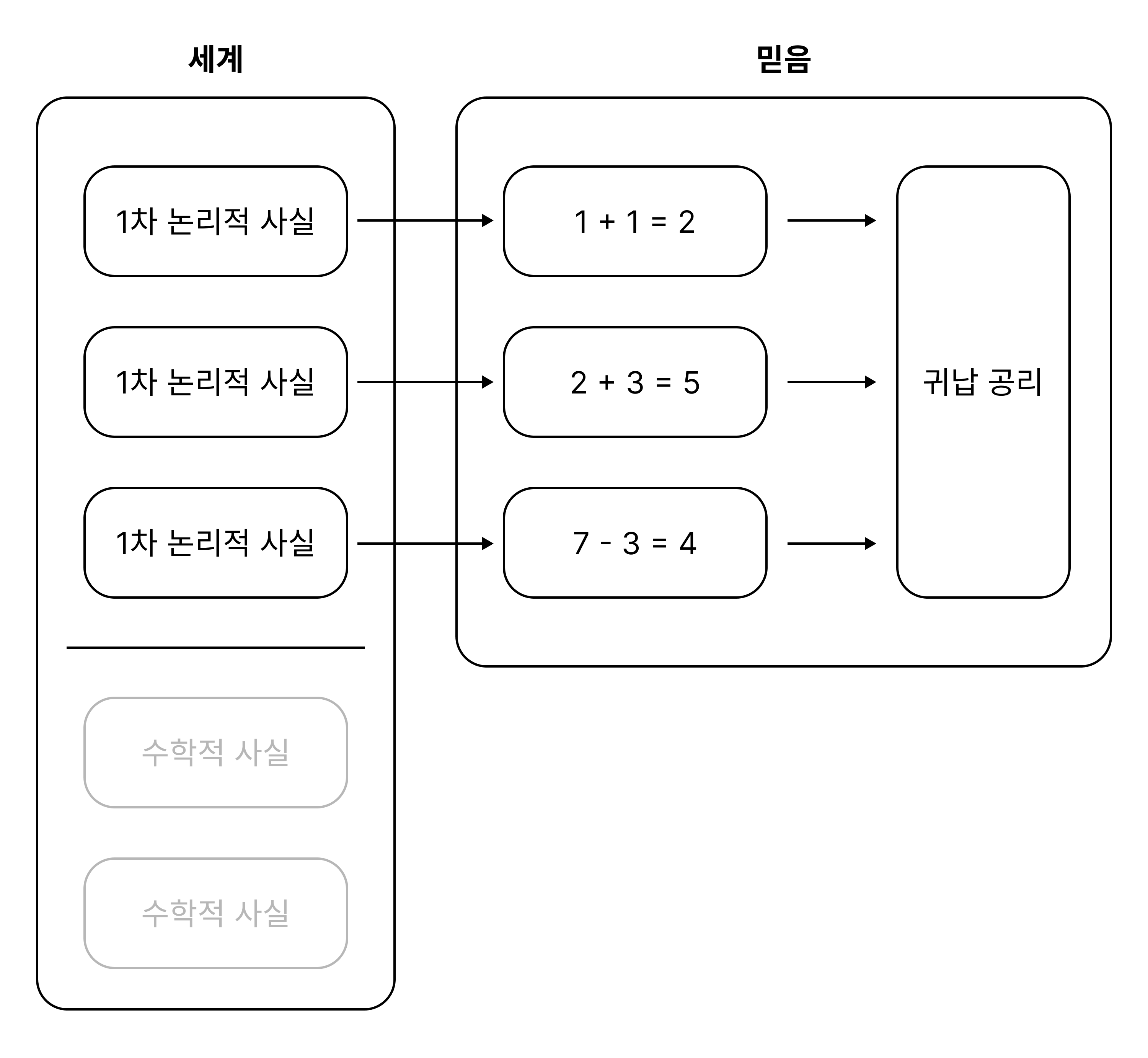
여기서 저자는 짧게 다음의 질문을 제시한다. 그렇다면 지금까지의 논의는 우리가 참인 1차 논리적 믿음들을 가지도록 진화했다는 것을 보여주는가? 저자는 이 질문의 답이 “아니오”일 것이라고 생각한다. 왜냐하면 논리적 사실들은 5 + 7 = 12와 같은 단순한 산술적 사실만 되어도 굉장히 복잡해지기 때문이다. 따라서 진화론적으로는 단순히 수학적 믿음을 가지는 개체가, 수학적 믿음, 논리적 믿음, 그리고 각각의 수학적 명제를 논리적 명제로 어떻게 번역할지에 관한 믿음을 가지는 개체보다 유리할 것으로 보인다. 즉, 논리적 사실들이 달랐더라면 우리의 수학적 믿음들 또한 달라졌을 것이지만 우리의 논리적 믿음들이 어떻게 되었을지는 불분명하다(— 라고 저자는 생각하는 듯한데, 사실 이 부분에 관한 저자의 코멘트가 너무 함축적이라서 잘 모르겠다. 논리적 믿음의 형성을 진화론적으로 설명할 수 없다는 별도의 논증으로 필자의 소논문을 참고하라.)
4. 또다른 수학은 상상 가능한가?
수학에 대한 진화적 설명을 기각한 저자는 자명한 설명으로 논의를 돌린다. 자명한 설명은, 현재의 수학적 사실들이 유일하게 가능한 수학적 사실들임을 주장한다.
통상적으로 윤리에 대한 자명한 설명은 설득력이 없는 것으로 간주되었다. 왜냐하면 윤리의 영역에서는 충분히 합리적인 개인들이 상충하는 입장을 가지는 경우가 자주 있기 때문이다. 서로 다른 윤리적 사실을 견지하는 합리적 개인들이 존재한다면, 현실과 다른 윤리적 사실을 가진 세계는 충분히 정합적으로 상상될 수 있다. 반면 수학의 경우에는 그런 상충이 거의 보이지 않는다. 트롤리 딜레마와 피타고라스 정리에 대한 사람들의 견해차를 비교해 보라.
그러나 저자는 이것이 윤리 실재론자에게 불리하도록 선별된 비교라고 주장한다. 우리는 윤리 실재론자들 사이에서 이견이 없는 명제들 — 이를테면 “아이를 재미로 고문하는 것은 정당하지 않다” — 을 찾을 수 있다. 반대로, 수학 실재론자들 사이에서 이견이 있는 수학의 공리들 또한 찾을 수 있다. 유한주의는 임의의 자연수보다 큰 자연수가 언제나 존재한다는 공리를 부정하고, 선택 공리는 전통적으로 굉장히 많은 논란을 야기했으며, 연속체 가설은 지금까지도 논란이 되고 있다. 따라서 저자는 현실과 다른 윤리적 참을 가지는 세계를 상상할 수 있는 것과 같은 정도로, 현실과 다른 수학적 참을 가지는 세계 — 이를테면 무한집합이 존재하지 않는 세계 — 를 상상할 수 있다고 주장한다.
5. 결론
저자는 진화론 논변이 윤리 실재론을 위협하는 것으로 여겨졌지만, 동일한 위협이 수학 실재론에도 가해짐을 논증했다. 저자는 수학 실재론 말고 오직 윤리 실재론만 위협하는 다른 논증이 있을 수도 있다는 사실을 인정한다. 일례로 하먼은 경험과학에서 수학의 필수불가결성indispensability으로부터 수학적 참을 경험적으로 정당화하는 콰인-퍼트넘 논증이 윤리에서는 적용되지 않는다는 점을 지적했다. 하지만 저자는 경험과학-수학 불가결성에 대한 근래의 회의주의와 경험과학-윤리 불가결성에 대한 새로운 논증들, 그리고 베나세라프 등의 인식론적 고려들을 제시하며, 수학 실재론과 윤리 반실재론을 동시에 견지하는 것이 점점 어려워지고 있음을, 어쩌면 불가능해질지도 모른다고 결론 내린다.
-
윤리적 문장은 감정의 발화라는 입장. 이 입장은 윤리학을 환호 및 야유와 동일시한다. 예를 들어 “도둑질은 나쁘다”는 “도둑질 우우!”와 동등하다 (“나는 도둑질을 싫어한다”와 동등하지는 않음에 유의하라). ↩
-
모든 윤리적 문장은 거짓이라는 입장. 이 입장은 윤리학을 플로지스톤 이론과 동일시한다. 플로지스톤이 존재하지 않으므로 플로지스톤 이론의 모든 문장이 틀렸듯이, 선함이 존재하지 않으므로 윤리학의 모든 문장은 틀렸다. ↩
-
인간의 정신이 윤리적 대상과 속성을 구성한다는 입장. 이 입장은 윤리학을 색깔 이론과 동일시한다. 색깔 이론의 객관성과 유용성과는 별개로 모든 인간이 사라지면 색의 개념도 사라지듯이, 모든 인간이 사라지면 선함의 개념도 사라진다. ↩
-
모든 윤리적 문장에는 생략된 전제구가 있다는 입장. 예를 들어 “트롤리의 선로를 바꿔야 한다”에서 생략된 전제구가 “공리주의에 따르면”이라면 이 문장은 참이고, “의무론에 따르면”이라면 거짓이다. ↩
-
수학은 규칙이 정해진 게임 활동이라는 입장. 이 입장은 수학을 체스의 수와 동일시한다. 가령 “1 + 1” 뒤에 “= 2”를 쓰는 것은 킹과 룩 사이를 비운 뒤 캐슬링을 하는 행위와 동등하다 (“킹과 룩 사이가 비어 있으면 캐슬링이 가능하다”와 동등하지는 않음에 유의하라). ↩
-
모든 수학적 문장은 거짓이라는 입장. 주석 2 참조. 필드는 유명론과 허구주의를 견지하면서도 수학이 과학에 유용할 수 있는 이유를 “다리 원리”를 통해 설명할 수 있다고 주장했다. ↩
-
인간의 정신이 수학적 대상과 속성을 구성한다는 입장. 주석 3 참조. 브라우어르의 구성주의는 수학이 인간의 시공간 인식에 정초되어야 한다고 주장한다. ↩
-
모든 수학적 명제에는 생략된 전제구가 있다는 입장. 예를 들어 “삼각형의 세 내각의 합은 180도이다”에서 생략된 전제구가 “유클리드 기하학에서”라면 이 문장은 참이고, “쌍곡 기하학에서”라면 거짓이다. ↩
Are Mathematics and Ethics in the Same Boat?: The Evolutionary Challenge
07 Nov 2025This post was originally written in Korean, and has been machine translated into English. It may contain minor errors or unnatural expressions. Proofreading will be done in the near future.
This article summarises Justin Clarke-Doane’s Morality and Mathematics: The Evolutionary Challenge (2012). “The author” refers to the author of the paper, while “the writer” refers to the author of this post. To avoid confusion between “morality” and “ethics,” the term “ethics” is used consistently throughout.
Overview
One of the objections to ethical realism is the evolutionary challenge. According to this argument, the ethical beliefs held by modern humans were shaped by evolutionary pressures. However, the principles of evolution are independent of ethical facts, meaning that even in a counterfactual world with entirely different ethical facts, humans would have evolved to hold the same ethical beliefs. Therefore, if our ethical beliefs are true, it would be an extraordinary coincidence that they align with the outcomes of evolution. Proponents of the evolutionary challenge argue that ethical realists must either accept this extraordinary coincidence or concede that we have no grounds to believe our ethical beliefs are true.
For instance, the reason we hold the ethical belief “we should care for others” is likely because, in human evolution, groups that valued mutual cooperation had higher survival rates than those that prioritised selfishness. However, the fact that mutual cooperation increases survival rates is not an ethical fact but a game-theoretic or mathematical fact. Thus, even if selfishness were ethically superior to mutual cooperation, we would still have evolved to believe “we should care for others.”
On the other hand, the evolutionary challenge has traditionally been seen as not threatening mathematical realism. This is because the principles of evolution appear to depend on mathematical truths. For example, individuals who believe that 1 + 1 = 2 are more likely to survive than those who do not, precisely because 1 + 1 = 2 is actually true. Joyce explains this as follows:
Suppose there is one lion behind bush A and another lion behind bush B. Our ancestors, P and Q, are hiding behind bush C. P believes that one lion plus another lion equals two lions, while Q believes that one lion plus another lion equals zero lions. P is less likely to die and more likely to pass on their genes than Q. This is because P is less likely than Q to step out from behind bush C and be eaten by the two lions. However, the explanation for this fact [italicised fact] presupposes that one lion plus another lion is actually two lions and not zero lions.
However, the author of the paper argues that this reasoning is mistaken. They claim that the evolutionary challenge threatens mathematical realism to the same extent that it threatens ethical realism. Ultimately, the author asserts that accepting either ethical realism or mathematical realism while rejecting the other is an incoherent position.
1. What Exactly Is Realism?
Before delving into the argument, the author seeks to clarify what is meant by ethical realism and mathematical realism. Generally, the author defines D-realism for a domain of discourse D as the conjunction of the following four positions:
- D-Truth-Aptness. Sentences in D have truth values.
- D-Truth. Some atomic or existentially quantified sentences in D are true.
- D-Independence. The truth values of sentences in D are independent of minds and language in a meaningful sense.
- D-Literalness. Sentences in D should be taken literally.
When D is set to ethics, (1) rules out Ayer’s emotivism, (2) rules out Mackie’s error theory, (3) rules out constructivism, and (4) rules out Harman’s relativism. When D is set to mathematics, (1) rules out Hilbert’s formalism, (2) rules out Field’s fictionalism, (3) rules out Brouwer’s constructivism, and (4) rules out if-thenism.
This paper assumes both ethical realism and mathematical realism and examines whether they can withstand the evolutionary challenge. Additionally, it assumes that most of our ethical and mathematical beliefs are true.
2. The Evolutionary Challenge to Ethical Realism
Having clarified the requirements of realism, let us examine how the evolutionary challenge attacks ethical realism. The challenge is based on the following premise:
Strong Premise. Our ethical beliefs were shaped by evolutionary pressures that are independent of their truth.
The strong premise consists of the following two sub-premises:
E. Our ethical beliefs were shaped by evolution.
NTT. The evolution of ethical beliefs occurred in a non-truth-tracking manner.
The precise meaning of NTT is captured by the following counterfactual conditional:
P. Suppose all other facts remained the same, but ethical facts were entirely different. Even so, we would have evolved to hold the same ethical beliefs that are true in the actual world.
Some might argue that Q could serve as an alternative interpretation of NTT:
Q. We could have evolved to hold false ethical beliefs.
However, the author contends that Q is untenable. While Darwin noted that if humans had evolved in an environment like that of bees, they might have condoned the killing of brothers by unmarried females, this example does not substantiate Q. To substantiate Q, one would need the additional assumption that “in a bee-like environment, it would have been wrong for unmarried females to kill their brothers,” which is not self-evident. (Consider the differing ethical weight of infanticide in premodern societies with frequent famine versus modern societies.) Thus, the author argues that Q can only be substantiated by presenting cases where individuals hold fundamentally false ethical beliefs, such as “pain is good” or “pleasure is bad.” However, individuals who believe that pain is good and pleasure is bad would have been evolutionarily eliminated, making Q untenable. Therefore, P is the correct interpretation of NTT.
However, P also faces challenges. Many ethical realists argue that ethical properties are metaphysically necessarily identical to descriptive properties. For instance, if “pleasure is good” is true, this truth is metaphysically necessary. According to this view, it is metaphysically impossible for descriptive facts to remain fixed while ethical facts change. Thus, the following interpretation of P is untenable:
P1. In a metaphysical sense, suppose all other facts remained the same, but ethical facts were entirely different. Even so, we would have evolved to hold the same ethical beliefs that are true in the actual world.
Instead, the author argues that P should be understood as follows:
P2. Suppose all other facts remained the same, but ethical facts were entirely different. We can intelligibly imagine such a scenario. Even so, we would have evolved to hold the same ethical beliefs that are true in the actual world.
To illustrate, consider a child who guesses the answer to the problem of finding $\zeta(-1)$ as $-1/12$ and gets it right. Since $\zeta(-1) = -1/12$ is metaphysically necessary, the counterfactual statement “even if the answer to this problem were different, the child would still have guessed correctly (the child’s answer was truth-tracking)” is metaphysically vacuous. Nevertheless, we can imagine a scenario where $\zeta(-1) \neq -1/12$, and in such an imagined scenario, the child would have been wrong. In this sense, the child’s answer was non-truth-tracking.
With the meanings of E and NTT clarified, let us examine how the strong premise leads to a refutation of ethical realism. Street and others present the following argument:
- Even if it is metaphysically impossible for ethical facts to be entirely different, we can imagine such a scenario.
- As far as we can imagine, even if ethical facts were entirely different, the ethical beliefs shaped by evolution would remain the same.
- Therefore, the fact that we hold true ethical beliefs in the actual world is an unexplained coincidence.
However, the author argues that (2) does not necessarily lead to (3). To derive (3) from (2), the following general principle must be assumed:
If the fundamental facts of D were different, then the truth of the D-beliefs that remain unchanged is coincidental.
The author provides the following counterexample to this principle. Chulsoo sees a basketball flying towards him and believes, “a basketball is flying towards me.” Here, it is metaphysically necessary that a basketball is identical to atoms arranged basketballwise. However, we can imagine a world where matter is composed of something other than atoms. Even in such a world, if a basketball were flying towards Chulsoo, he would hold the same belief, “a basketball is flying towards me.” Thus, even if the fundamental facts about basketballs were different, Chulsoo would hold the same belief, yet the truth of his belief in the actual world is not coincidental.
Writer’s note: I believe the author has provided a flawed analogy. The belief “a basketball is flying towards me” held by Chulsoo in a world where basketballs are composed of atoms is not the same as the belief held by Chulsoo in a world where basketballs are composed of continua. This is because the meaning of “basketball” for the two Chulsoos is determined by ostension. In the former case, “basketball” refers to “atoms arranged basketballwise,” while in the latter, it refers to “continua condensed basketballwise.” Thus, if the fundamental facts about basketballs change, Chulsoo would hold a different belief. In contrast, the meaning of ethical language does not seem to be determined by ostension.
Nevertheless, the author argues that even if Street’s argument does not demonstrate the complete impossibility of explaining why we hold true ethical beliefs, it at least shows that the following two explanations are flawed:
- Evolutionary Explanation. We hold true ethical beliefs because we were selected to hold true ethical beliefs.
- Trivial Explanation. We hold true ethical beliefs because the current ethical facts are the only possible ethical facts, and believing those facts is evolutionarily advantageous.
Focus on the distinction between the evolutionary explanation and the trivial explanation. The evolutionary explanation claims that if ethical facts had changed — even if only in an imaginable sense — we would have evolved to believe those changed facts. In contrast, the trivial explanation asserts that it is impossible for ethical facts to change, either metaphysically or imaginably, and therefore, it suffices to explain how evolution produced beings that believe the actual ethical facts.
Writer’s note: The trivial explanation seems to presuppose the game-theoretic explanation mentioned in the overview. That is, the trivial explanation attempts to overcome the evolutionary challenge to ethical realism by relying on (i) the strong necessity of ethical facts, (ii) the mathematical fact that those ethical facts are evolutionarily advantageous, and (iii) the necessity of mathematical facts. This appears to ground the explanation of the truth of ethical beliefs in the explanation of the truth of mathematical beliefs.
However, if the purpose of the evolutionary challenge is to argue that the evolutionary explanation and the trivial explanation are flawed, then the challenge does not need to assume E ∧ NTT but only E → NTT. Thus, the evolutionary challenge can be summarised as follows:
Evolutionary Challenge. If E → NTT, then explaining why we hold true ethical beliefs through the evolutionary explanation or the trivial explanation is flawed.
The author summarises the evolutionary challenge in this way and then examines how valid it is in the context of mathematics.
3. Does Mathematics Influence Evolution?
It is commonly thought that mathematics is not subject to the evolutionary challenge. Unlike ethical truths, which are independent of evolution (ethical truths can change without affecting evolution), mathematical truths are thought to influence evolution. Let us revisit Joyce’s example:
Suppose there is one lion behind bush A and another lion behind bush B. Our ancestors, P and Q, are hiding behind bush C. P believes that one lion plus another lion equals two lions, while Q believes that one lion plus another lion equals zero lions. P is less likely to die and more likely to pass on their genes than Q. This is because P is less likely than Q to step out from behind bush C and be eaten by the two lions. However, the explanation for this fact [italicised fact] presupposes that one lion plus another lion is actually two lions and not zero lions.
However, the author identifies two problems with Joyce’s argument. The first problem arises from the principle underlying Joyce’s argument:
If the evolutionary explanation for why we hold certain beliefs about D presupposes the content of those beliefs, then we were selected to hold true beliefs about D.
The author argues that even if we were not selected to hold true D-beliefs (i.e., our D-beliefs are false or non-truth-tracking), the evolutionary explanation for our D-beliefs can still presuppose the content of those beliefs. For instance, all types of explanations presuppose the content of our logical beliefs, yet it remains questionable whether we were selected to hold true logical beliefs (see the writer’s short paper).
Even so, one might counter by adopting Quine-Putnam-style holistic epistemology, arguing that the consideration that mathematical facts explain our mathematical beliefs can serve as a provisional justification for the truth of those mathematical facts. In response, the author identifies a second, more serious problem: the evolutionary explanation for our mathematical beliefs is not actually related to mathematical facts. Instead, the author argues that the evolutionary explanation is only related to first-order logical facts. In the earlier example of the lions, the reason P is more likely to survive than Q is not because M is true but because L is true:
M. 1 + 1 = 2
L. If there is one lion behind bush A, one lion behind bush B, and no lion behind bush A is the same as any lion behind bush B, then there are two lions behind bushes A and B.
L can be expressed as the following first-order logical formula:
\[\begin{align} &\;\exists! x A(x) \land \exists! y B(y) \land \forall x, y (A(x) \land B(y) \rightarrow x \neq y) \\ &\rightarrow \exists x, y \big((x \neq y) \land (A(x) \lor B(x)) \land (A(y) \lor B(y)) \\ &\quad \quad \land\; \forall z ( (A(z) \lor B(z)) \rightarrow (z = x) \lor (z = y))\big) \end{align}\]While many mathematicians and philosophers hold that mathematics can be reduced to logic, no one claims that the reduction ends at first-order logic. Therefore, if the evolutionary explanation for our mathematical beliefs depends only on first-order logical facts and not on mathematical facts, it cannot definitively or provisionally conclude that we were selected to hold true mathematical beliefs.
Moreover, mathematical realists cannot simply identify M with L. This is because one of the requirements of realism is D-literalness. The statement 1 + 1 = 2 must be taken literally, and when taken literally, it asserts the existence of the numbers 1 and 2 and a specific relationship between them under addition.
In conclusion, the reason P is more likely to survive than Q is not because the content of P’s mathematical belief M is true but because the corresponding logical content L is true. The correspondence between M and L can be explained without assuming mathematical objects. Various anti-realist positions mentioned earlier — formalism, fictionalism, constructivism, if-thenism — all explain the correspondence between M and L without positing mathematical entities.
Of course, we also hold mathematical beliefs that cannot be captured by first-order logic. Belief in the induction axiom is one example. However, the author points out that belief in the induction axiom was not directly shaped by evolutionary pressures. The induction axiom was not explicitly formulated until the 17th century. Belief in the induction axiom arose from formalising basic arithmetic beliefs. In other words, we believe in the induction axiom because of our beliefs in basic arithmetic, which were shaped by first-order logical facts, not mathematical facts. Consequently, mathematical facts that transcend logic have no influence on the evolutionary formation of mathematical beliefs (see the following diagram: A → B means “A causes the evolution of beings that believe B”).
Here, the author briefly raises the following question: does the preceding discussion show that we were selected to hold true first-order logical beliefs? The author thinks the answer is “no.” This is because logical facts become exceedingly complex even for simple arithmetic facts like 5 + 7 = 12. Evolutionarily, it seems more advantageous for beings to simply hold mathematical beliefs than to hold mathematical beliefs, logical beliefs, and beliefs about how to translate each mathematical statement into a logical statement. Thus, while logical facts might influence the evolution of our mathematical beliefs, it remains unclear how they influenced the evolution of our logical beliefs (— or so the author seems to think, though their comments on this point are too terse to be clear. For a separate argument on why the formation of logical beliefs cannot be explained evolutionarily, see the writer’s short paper).
4. Is Another Mathematics Imaginable?
Having dismissed the evolutionary explanation for mathematics, the author turns to the trivial explanation. The trivial explanation asserts that the current mathematical facts are the only possible mathematical facts.
It is commonly thought that the trivial explanation is unconvincing in ethics. This is because, in ethics, sufficiently reasonable individuals often hold conflicting positions. If rational individuals can hold different ethical facts, then worlds with different ethical facts are imaginably coherent. In contrast, such conflicts are rarely observed in mathematics. Compare the divergence of opinions on the trolley dilemma with the consensus on the Pythagorean theorem.
However, the author argues that this comparison is biased against ethical realists. We can find ethical propositions on which ethical realists unanimously agree — for instance, “it is wrong to torture children for fun.” Conversely, we can also find mathematical axioms on which mathematical realists disagree. Finitism denies the axiom that there is always a natural number greater than any given natural number, the