Completeness Theorem and Löwenheim-Skolem Theorem

10 Apr 2025

This post was originally written in Korean, and has been machine translated into English. It may contain minor errors or unnatural expressions. Proofreading will be done in the near future.

Gödel’s completeness theorem and the Löwenheim-Skolem theorem are amongst the most fundamental theorems in mathematical logic. To consolidate the fundamentals, I have revisited the proofs of these theorems. In this article, $T$ is considered as a first-order logical theory in language $\mathcal{L}$.

Gödel’s Completeness Theorem

Gödel’s Completeness Theorem. If $T \vDash \phi$, then $T \vdash \phi$.

Proof

We prove the following equivalent statement. (Exercise: Why is this equivalent?)

If $T$ is a consistent theory, then $T$ has a model.

1. Extending $\mathcal{L}$ to the Skolem language $\mathcal{L}_S$

Let $\kappa = \mathrm{max}(\aleph_0, |\mathcal{L}|)$. Let $\mathcal{L}_S$ be the language obtained by adding constants $\lbrace c_\alpha \rbrace _{\alpha \in \kappa}$ (where $\alpha$ is an ordinal) to $T$. Here, the subscript $S$ indicates that each constant will serve as a Skolem constant.

2. Extending $T$ to the Henkin theory $T_H$

Since the size of the set of formulae in $\mathcal{L}_S$ with one free variable is equal to $\kappa$, by the well-ordering principle, we can represent them as $\lbrace P_\alpha \rbrace _{\alpha \in \kappa}$. From this, we define the following set of sentences:

\[\Sigma = \{ Q_\alpha := \exists x P_\alpha \rightarrow P_\alpha(c_\lambda) \mid \alpha \in \kappa \}\]

where $c_\lambda$ is the constant with the smallest index amongst the constants that do not appear in $P_\alpha$ and $Q_\beta \; (\beta < \alpha)$ (the existence of such a constant is guaranteed by the fact that ordinals are well-ordered). Now we define $T_H = T \cup \Sigma$. We call $T_H$ the Henkin theory and $Q_\alpha$ the Henkin axioms.

3. Extending $T_H$ to a maximally consistent theory $\overline{T_H}$

Lindenbaum’s Lemma. When $T$ is a consistent theory, there exists a maximally consistent theory $\overline{T}$ that extends $T$. That is, $T \subseteq T’$ and for any $\mathcal{L}$ sentence $\phi$, either $\phi \in \overline{T}$ or $\lnot\phi \in \overline{T}$.

Proof. We order the collection of consistent theories that extend $T$ by $\subseteq$ and apply Zorn’s lemma.

When $T$ is a consistent theory, we can easily show that $T_H$ is also consistent. Therefore, by Lindenbaum’s lemma, there exists a maximally consistent theory $\overline{T_H}$ that extends $T_H$.

4. Defining the canonical model of $\overline{T_H}$

Let $c_\alpha \sim c_\beta$ be the relation that holds when $(c_\alpha = c_\beta) \in \overline{T_H}$. From the fact that $\overline{T_H}$ is a consistent theory, we can show that $\sim$ is an equivalence relation. Therefore, the equivalence classes $[c_\alpha]$ of constants are well-defined. We now define a structure $\mathfrak{M}$ for $\mathcal{L}_S$ as follows:

1. Constants: $c_\alpha^{\mathfrak{M}} = [c_\alpha]$
2. Predicates: $R^{\mathfrak{M}}(c_{\alpha_1}^\mathfrak{M}, \dots, c_{\alpha_n}^{\mathfrak{M}}) \iff \overline{T_H} \vdash R(c_{\alpha_1}, \dots, c_{\alpha_n}) $
3. Functions: $f(c_\alpha^\mathfrak{M}) = c_\beta^\mathfrak{M} \iff T_H \vdash \exists x (f(c_\alpha) = x) \rightarrow f(c_\alpha) = c_\beta$

Since $\overline{T_H}$ is maximally consistent, (2) is well-defined, and since it is a Henkin theory, (3) is well-defined. Therefore, $\mathfrak{M}$ is well-defined, and we can easily verify that $\mathfrak{M}$ is a model of $\overline{T_H}$. Since $\mathfrak{M}$ is also a model of $T$, $T$ has a model. ■

Remark 1. The proof of the completeness theorem depends on the axiom of choice in that it uses the well-ordering principle and Zorn’s lemma. It can also be proved using weaker forms of the axiom of choice such as König’s lemma or the axiom of dependent choice.

Remark 2. The compactness theorem is obtained as a corollary of the completeness theorem. (Exercise)

Remark 3. The size of the model constructed in the proof of the completeness theorem does not exceed $\kappa = \mathrm{max}(\aleph_0, |\mathcal{L}|)$. Since we take equivalence classes in the final step, there is no guarantee that it equals $\kappa$.

Löwenheim-Skolem Theorem

Löwenheim-Skolem Theorem. Suppose $T$ has an infinite model. For any $\kappa \geq \mathrm{max}(\aleph_0, |\mathcal{L}|)$, there exists a model of $T$ of size $\kappa$.

Proof

Downward Löwenheim-Skolem Theorem

Downward Löwenheim-Skolem Theorem. $T$ has a model of size not exceeding $\mathrm{max}(\aleph_0, |\mathcal{L}|)$.

Proof. This follows immediately from Remark 2. □

Upward Löwenheim-Skolem Theorem

Upward Löwenheim-Skolem Theorem. Suppose $T$ has an infinite model. For any infinite cardinal $\kappa$, there exists a model of $T$ of size at least $\kappa$.

Proof. Let $\mathcal{L}’$ be the language obtained by adding constants $\lbrace c_\alpha \rbrace _{\alpha \in \kappa}$ to $\mathcal{L}$. Define the following set of $\mathcal{L}’$-sentences:

\[\Sigma = \{ c_\alpha \neq c_\beta : \alpha, \beta \in \kappa, \alpha \neq \beta \}\]

Let $T’ = T \cup \Sigma$. Since $T$ has an infinite model $\mathfrak{M}$, any finite subtheory of $T’$ is satisfied by $\mathfrak{M}$. Therefore, by the compactness theorem, $T’$ is consistent, and by the completeness theorem, it has a model. Since $\Sigma$ requires that any model of $T’$ has at least $\kappa$ elements, $T’$ has a model of size at least $\kappa$, and thus $T$ also has a model of size at least $\kappa$. □

Löwenheim-Skolem Theorem

Let $\kappa \geq \mathrm{max}(\aleph_0, |\mathcal{L}|)$. Define $\mathcal{L}’$ and $T’$ as above.

Since $\mathrm{max}(\aleph_0, |\mathcal{L}’|) = \kappa$, by the downward Löwenheim-Skolem theorem, $T’$ has a model of size not exceeding $\kappa$. However, as pointed out in the proof of the upward Löwenheim-Skolem theorem, every model of $T’$ has size at least $\kappa$. Therefore, $T’$ has a model of size exactly $\kappa$, and thus $T$ also has a model of size exactly $\kappa$. ■

자이페르트-판 캄펀 정리에 대한 노트

04 Apr 2025

위상공간 $X$의 열린 덮개 $U, V$를 생각하자. 위상공간들의 범주 $\mathbf{Top}$에서 다음 푸시아웃_pushout 도식의 극한은 $X$이다.

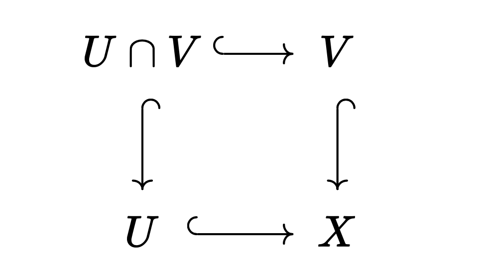
자이페르트-판 캄펀 정리는, $U, V$가 경로 연결_{path connected}이고 $x_0 \in U \cap V$일 때, 위 극한이 함자 $\pi_1(-, x_0): \mathbf{Top} \to \mathbf{Grp}$에 대해 보존된다는 내용이다.

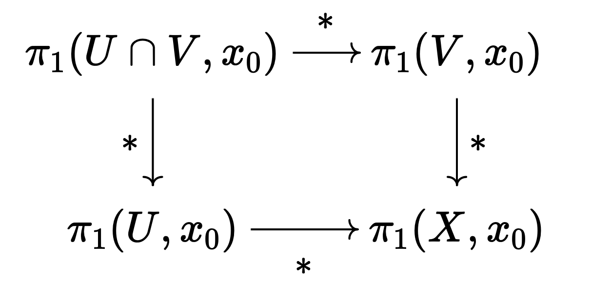
그런데 푸시아웃의 극한은 왼쪽 도식의 쌍대 극한_colimit이다. 만약 $I$에 대응되는 대상이 초기 대상_{initial object}이라면, 사상 $I \to J, J \to K$는 유일하게 결정되므로 사실상 왼쪽 도식의 쌍대 극한은 오른쪽 도식의 쌍대 극한과 같으며, 이는 범주론적 합에 해당한다.

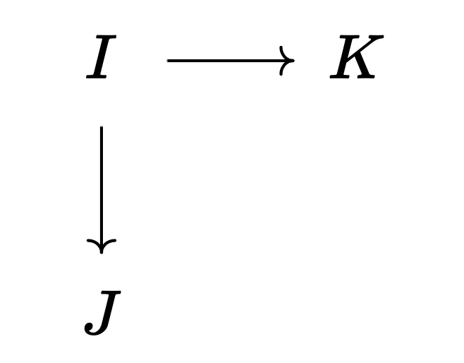
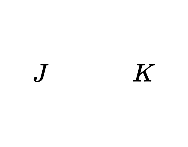
$\mathbf{Grp}$의 초기 대상은 자명군_{trivial group}이며, 범주론적 합은 자유곱이다. 이에 따라 $U \cap V$가 단순 연결 공간일 때, $\pi_1(X)$는 $\pi_1(U)$와 $\pi_1(V)$의 자유곱이라는 결론을 얻는다.

Notes on the Seifert-van Kampen Theorem

04 Apr 2025

This post was originally written in Korean, and has been machine translated into English. It may contain minor errors or unnatural expressions. Proofreading will be done in the near future.

Consider an open cover $U, V$ of a topological space $X$. In the category of topological spaces $\mathbf{Top}$, the limit of the following pushout diagram is $X$.

The Seifert-van Kampen theorem states that when $U, V$ are path connected and $x_0 \in U \cap V$, the above limit is preserved under the functor $\pi_1(-, x_0): \mathbf{Top} \to \mathbf{Grp}$.

However, the limit of a pushout is the colimit of the left diagram. If the object corresponding to $I$ is an initial object, then the morphisms $I \to J, J \to K$ are uniquely determined, so the colimit of the left diagram is essentially the same as the colimit of the right diagram, which corresponds to the categorical sum.

The initial object in $\mathbf{Grp}$ is the trivial group, and the categorical sum is the free product. Accordingly, when $U \cap V$ is a simply connected space, we obtain the conclusion that $\pi_1(X)$ is the free product of $\pi_1(U)$ and $\pi_1(V)$.

범주론적 관점에서의 곱 위상·상자 위상과 직곱·직합의 차이

02 Apr 2025

곱 위상과 상자 위상

학부 위상에서 곱 위상_{product topology}과 상자 위상_{box topology}을 다루는 부분은 많은 학생에게 난관으로 다가오는 대목이다. 겉보기에는 상자 위상이 훨씬 직관적인데, 교재에서는 상자 위상보다 곱 위상이 다루기에 자연스러운 개념이라고 가르치기 때문이다.

정의. 위상공간의 모임 $\lbrace X_i \rbrace _{i \in I}$에 대해, 상자 위상공간 $\prod X_i$는 다음의 기저로 생성되는 위상공간이다.

\[\left\{ \prod U_i : U_i \text{ is open in } X_i \right\}\]

정의. 위상공간의 모임 $\lbrace X_i \rbrace _{i \in I}$에 대해, 곱 위상공간 $\prod X_i$는 다음의 기저로 생성되는 위상공간이다.

\[\left\{ \prod U_i : U_i \text{ is open in } X_i,\; U_i \neq X_i \text{ for only finitely many } i\right\}\]

일례로 $\mathbb{R}^\omega$에서 $(1, 1, 1, \dots)$의 근방은 각각 다음과 같다.

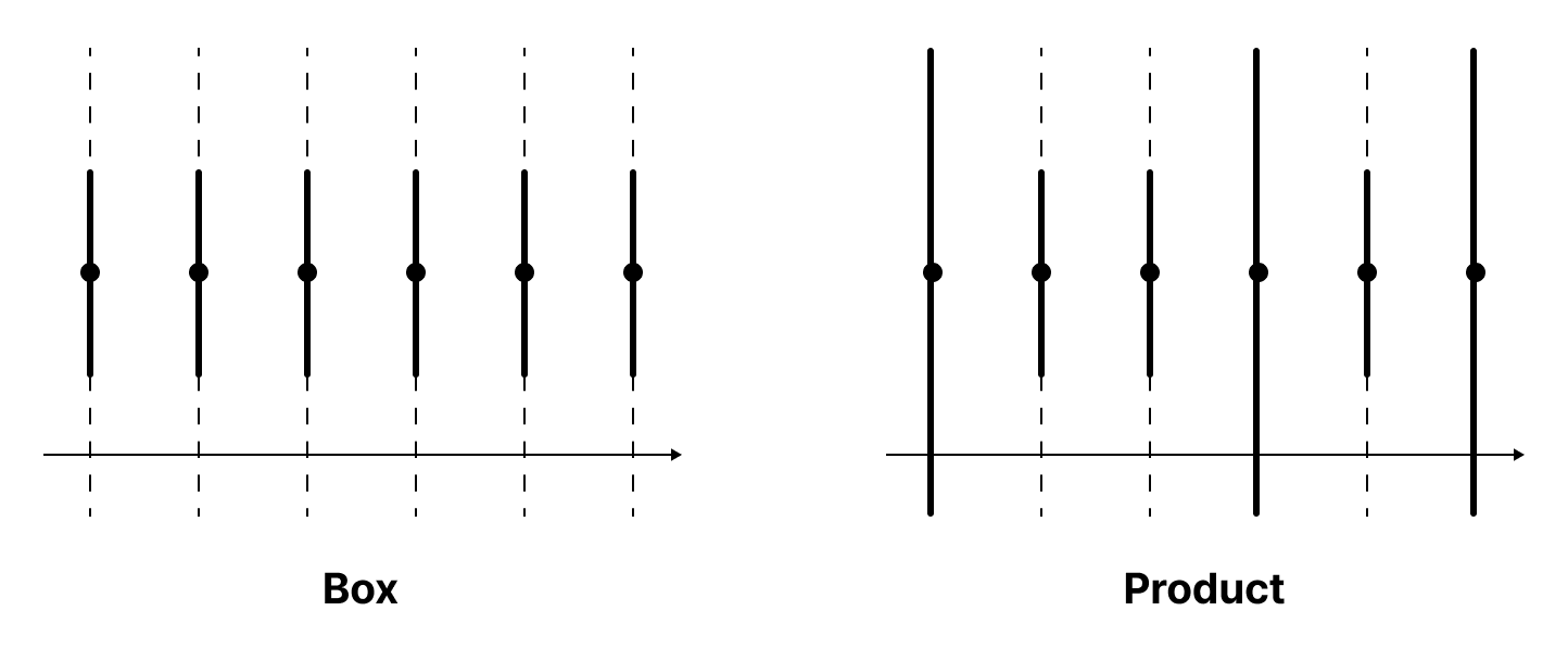
왜 곱 위상은 상자 위상보다 자연스러운 위상으로 간주될까? 그 이유는 범주론에서 대상의 곱을 정의하는 방법과 관련이 있다.

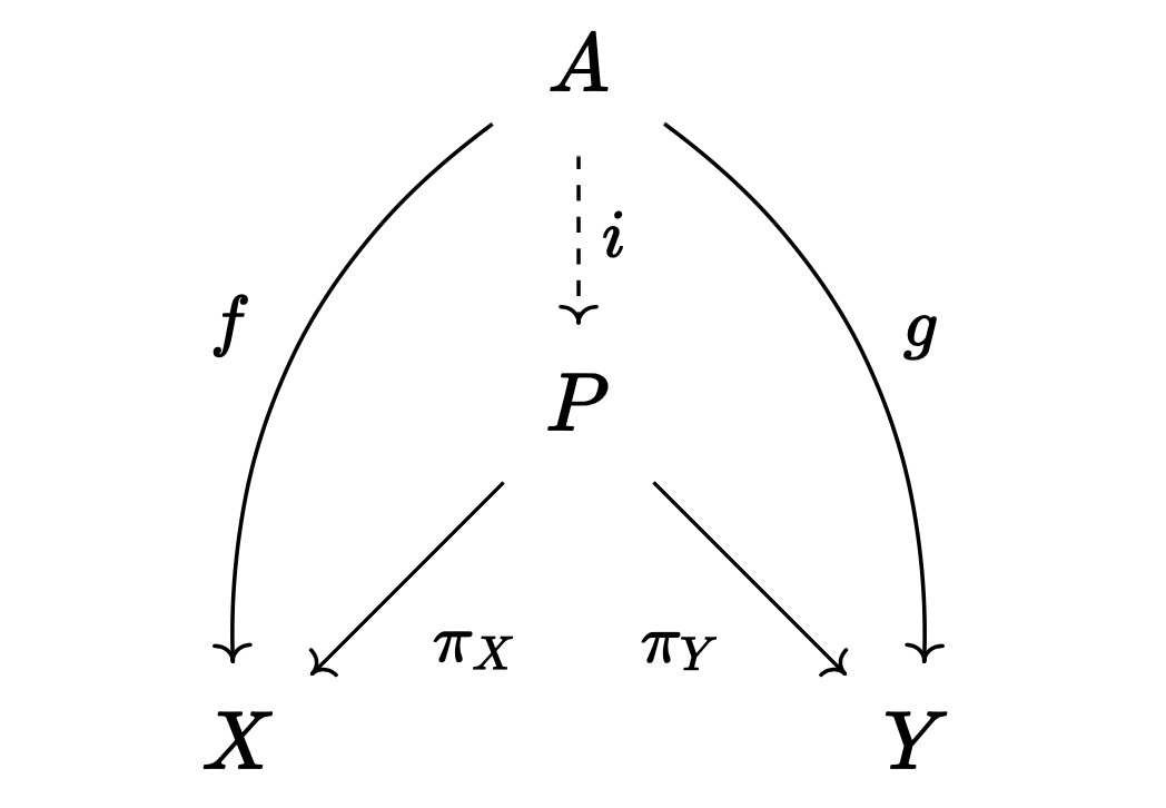
정의. $X, Y$가 범주 $\mathcal{A}$의 대상이라고 하자. $P \in \mathcal{A}$와 사상 $\pi_X : P \to X$, $\pi_Y : P \to Y$에 대해, 다음 조건이 만족될 때 $P$를 $X, Y$의 곱_product이라고 하며, $P = X \times Y$와 같이 적는다.

• 임의의 $A \in \mathcal{A}$와 $f: A \to X$, $g: A \to Y$에 대해 다음 도식이 가환이 되도록 하는 사상 $i: A \to P$가 언제나 유일하게 존재한다.

위의 정의는 자연스러운 방식으로 3개 이상, 또는 무한한 대상들의 곱으로 일반화된다. 극한_limit의 개념이 익숙한 독자라면, 곱은 이산 범주의 극한으로 이해할 수 있다. 또는, 곱은 주어진 대상들의 정보를 온전히 인코딩하는 가장 작은 범주로 이해할 수 있다.

집합들의 범주에서 곱은 곱집합과 같다. 특히 $\pi_X, \pi_Y$는 각각 $(x, y) \mapsto x$, $(x, y) \mapsto y$로 주어진다.

위상공간들의 범주에서 곱은 상자 위상이 아닌 곱 위상이다. 이는 다음의 정리로 보증된다.

정리. 사영함수 $\pi_k : \prod_{i \in I}X_i \to X_k$가 각 $k \in I$에 대해 연속이 되도록 하는 가장 작은 $\prod_{i \in I}X_i$의 위상은 곱 위상이다.

상자 위상도 각 사영함수가 연속이라는 특징을 가지지만, 상자 위상은 곱 위상보다 큰 토폴로지이다. 따라서 상자 위상은 범주론적 곱이 아니다.

상자 위상이 곱이 아님을 보이는 반례를 살펴보자. $\mathbb{R}^\omega$에 상자 위상을 부여하자. 만약 상자 위상이 범주론적 곱이라면, 임의의 연속인 $f_k: \mathbb{R} \to \mathbb{R}$에 대해 $\pi_k \circ i = f_k$가 되도록 하는 연속함수 $i : \mathbb{R} \to \mathbb{R}^\omega$가 존재해야 한다. $f_k: x \mapsto kx$라면 $i$는 $x \mapsto (x, 2x, 3x, \dots)$이다. 상자 위상에서는 $U = (0, 1)^\omega$가 열린 집합이므로, $i$가 연속이면 $i^{-1}(U)$가 열린집합이다. 그런데 $i^{-1}(U) = \lbrace 0 \rbrace $이므로, 상자 위상은 곱의 성질을 만족하지 않는다.

직곱과 직합

상자 위상과 곱 위상의 차이는 전체 공간이 아닌 인덱스가 유한한지의 여부에 있다. 이와 유사한 차이를 대수학에서도 발견할 수 있다.

정의. 벡터 공간들의 모임 $\lbrace V_i \rbrace _{i \in I}$에 대해, 직곱_{direct product} $\prod V_i$를 다음과 같이 정의한다.

\[\prod V_i = \left\{ (v_i)_{i \in I} : v_i \in V_i \right\}\]

정의. 벡터 공간들의 모임 $\lbrace V_i \rbrace _{i \in I}$에 대해, 직합_{direct sum} $\bigoplus V_i$를 다음과 같이 정의한다.

\[\bigoplus V_i = \left\{ (v_i)_{i \in I} : v_i \in V_i,\; v_i \neq 0 \text{ for only finitely many }i \right\}\]

벡터의 연산은 항별_term-wise로 정의한다. 또한 벡터 공간이 아닌 군에 대해서도 같은 방식으로 직곱과 직합을 정의할 수 있다.

직곱과 상자 위상, 직합과 곱 위상의 정의가 비슷하다는 점으로부터 직합이 범주론적 곱에 대응된다고 생각할 수 있지만 그렇지 않다. 대수의 경우 범주론적 곱에 대응되는 것은 직곱이다. 직합은 범주론적 곱의 조건을 일반적으로 만족하지 않는다.

일례로 다음의 경우를 보자. 일차원 실수 공간 $\mathbb{R}$의 직합 $\mathbb{R}^\omega$를 고려하자. 만약 직합이 범주론적 곱이라면, 임의의 선형인 $f_k: \mathbb{R} \to \mathbb{R}$에 대해 $\pi_k \circ i = f_k$가 되도록 하는 연속함수 $i : \mathbb{R} \to \mathbb{R}^\omega$가 존재해야 한다. $f_k: x \mapsto x$라면 $i$는 $x \mapsto (x, x, x, \dots)$이다. 그런데 $i(1) = (1, 1, 1, \dots) \notin \mathbb{R}^\omega$이므로, 직합은 곱의 성질을 만족하지 않는다.

대신 직합은 범주론적 합_sum에 대응된다. 범주론적 합은 곱의 켤레_dual이기 때문에 쌍곱_coproduct이라고도 한다.

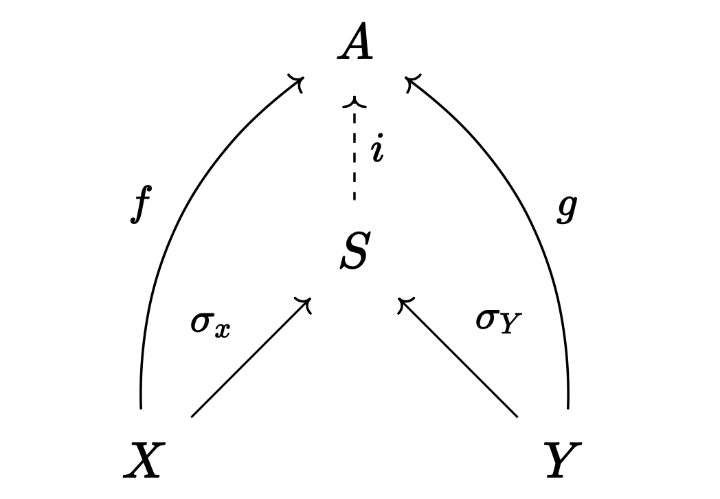
정의. $X, Y$가 범주 $\mathcal{A}$의 대상이라고 하자. $S \in \mathcal{A}$와 사상 $\sigma_X : X \to S$, $\sigma_Y : Y \to S$에 대해, 다음 조건이 만족될 때 $S$를 $X, Y$의 합_sum이라고 하며, $S = X + Y$와 같이 적는다.

• 임의의 $A \in \mathcal{A}$와 $f: X \to A$, $g: Y \to X$에 대해 다음 도식이 가환이 되도록 하는 사상 $i: S \to A$가 언제나 유일하게 존재한다.

앞서 들었던 예시를 다시 보자. 직합 $\bigoplus_\omega \mathbb{R}$를 고려하자. $\sigma_k: \mathbb{R} \to \bigoplus_\omega \mathbb{R}$은 다음과 같이 주어진다.

\[x \mapsto (0, \dots, 0, x, 0, \dots) \quad \text{($x$ is at the $k$th index)}\]

$A = \mathbb{R}$이라고 하고, 항등사상 $f_k : \mathbb{R} \to \mathbb{R}$을 고려하자. $\bigoplus_\omega \mathbb{R}$가 범주론적 합이라면 $i \circ \sigma_k = f_k$가 되도록 하는 연속함수 $i : \bigoplus_\omega \mathbb{R} \to \mathbb{R}$가 존재해야 한다. 실제로 이는 다음과 같이 존재한다.

\[i: (x_i)_{i \in \omega} \mapsto \sum_{i \in \omega} x_i\]

$\bigoplus_\omega \mathbb{R}$의 원소는 오직 유한한 비자명 항을 가지므로 $i$는 잘 정의됨에 주목하라. 반면, 이 예시는 직곱 $\mathbb{R}^\omega$가 범주론적 합이 아님을 보여준다. 직곱의 경우 $i$가 잘 정의되지 않기 때문이다. 이는 $i$에 $(1, 1, 1, \dots)$를 대입해 보면 알 수 있다.

군의 경우 범주론적 곱과 범주론적 합에 대응되는 연산은 일반적인 군의 범주를 따지냐, 아벨군의 범주를 따지냐에 따라 조금 다르다. 이 부분은 간단한 노트 정도로 남겨둔다.

	대수적 정의	범주론적 정의
자유곱	형식적 단어의 집합 + 병치 연산	$\mathbf{Grp}$의 합
직합	유한한 비자명 항을 가지는 튜플의 집합 + 항별 연산	$\mathbf{Ab}$의 합
직곱	튜플의 집합 + 항별 연산	$\mathbf{Grp}$의 곱

The Difference Between Product and Box Topologies, and Direct Product and Direct Sum from a Categorical Perspective

02 Apr 2025

Product Topology and Box Topology

Product topology and box topology often stir confusion among many undergraduate students. For, although the box topology appears more intuitive at first glance, textbooks teach that the product topology is the more “natural” concept to work with.

Definition. For a collection of topological spaces $\lbrace X_i \rbrace _{i \in I}$, the box topological space $\prod X_i$ is the topological space generated by the following basis:

\[\left\{ \prod U_i : U_i \text{ is open in } X_i \right\}\]

Definition. For a collection of topological spaces $\lbrace X_i \rbrace _{i \in I}$, the product topological space $\prod X_i$ is the topological space generated by the following basis:

\[\left\{ \prod U_i : U_i \text{ is open in } X_i,\; U_i \neq X_i \text{ for only finitely many } i\right\}\]

For instance, the neighbourhoods of $(1, 1, 1, \dots)$ in $\mathbb{R}^\omega$ are as follows:

Why is the product topology considered more natural than the box topology? The reason is related to how products of objects are defined in category theory.

Definition. Let $X, Y$ be objects in category $\mathcal{A}$. For $P \in \mathcal{A}$ and morphisms $\pi_X : P \to X$, $\pi_Y : P \to Y$, we call $P$ the product of $X, Y$ and write $P = X \times Y$ when the following condition is satisfied:

• For any $A \in \mathcal{A}$ and morphisms $f: A \to X$, $g: A \to Y$, there exists a unique morphism $i: A \to P$ such that the following diagram commutes:

The above definition naturally generalises to products of three or more, or infinitely many objects. Readers familiar with the concept of limits will recognise that the product can be understood as the limit of a discrete category. Alternatively, the product can be understood as the smallest category that fully encodes the information of the given objects.

In the category of sets, the product coincides with the Cartesian product. In particular, $\pi_X, \pi_Y$ are given by $(x, y) \mapsto x$ and $(x, y) \mapsto y$ respectively.

In the category of topological spaces, the product is the product topology, not the box topology. This is seen by the following theorem:

Theorem. The smallest topology on $\prod_{i \in I}X_i$ such that the projection functions $\pi_k : \prod_{i \in I}X_i \to X_k$ are continuous for each $k \in I$ is the product topology.

while the box topology also has the property that each projection function is continuous, the box topology is a larger topology than the product topology. Therefore, the box topology is not the categorical product.

Let us examine a counterexample showing that the box topology is not the categorical product. Consider $\mathbb{R}^\omega$ with the box topology. If the box topology were the categorical product, then for any continuous functions $f_k: \mathbb{R} \to \mathbb{R}$, there would exist a continuous function $i : \mathbb{R} \to \mathbb{R}^\omega$ such that $\pi_k \circ i = f_k$. If $f_k: x \mapsto kx$, then $i$ would be $x \mapsto (x, 2x, 3x, \dots)$. In the box topology, $U = (0, 1)^\omega$ is an open set, so if $i$ were continuous, then $i^{-1}(U)$ would be an open set. However, $i^{-1}(U) = \lbrace 0 \rbrace $, so the box topology does not satisfy the property of a product. (Note that in the case of product topology, $U$ is not an open set.)

Direct Product and Direct Sum

The difference between the box topology and product topology lies in whether only finitely many indices are allowed to be non-trivial. A similar difference can be found in algebra.

Definition. For a collection of vector spaces $\lbrace V_i \rbrace _{i \in I}$, the direct product $\prod V_i$ is defined as follows:

\[\prod V_i = \left\{ (v_i)_{i \in I} : v_i \in V_i \right\}\]

Definition. For a collection of vector spaces $\lbrace V_i \rbrace _{i \in I}$, the direct sum $\bigoplus V_i$ is defined as follows:

\[\bigoplus V_i = \left\{ (v_i)_{i \in I} : v_i \in V_i,\; v_i \neq 0 \text{ for only finitely many }i \right\}\]

Vector operations are defined term-wise. The same definitions of direct product and direct sum can be applied to groups as well.

From the similarity between the definitions of direct product and box topology, and direct sum and product topology, one might think that the direct sum corresponds to the categorical product, but this is not the case. In algebra, the direct product corresponds to the categorical product. The direct sum does not generally satisfy the conditions of a categorical product.

Consider the following example: Let us examine the direct sum $\mathbb{R}^\omega$ of one-dimensional real spaces $\mathbb{R}$. If the direct sum were the categorical product, then for any linear maps $f_k: \mathbb{R} \to \mathbb{R}$, there would exist a continuous function $i : \mathbb{R} \to \mathbb{R}^\omega$ such that $\pi_k \circ i = f_k$. If $f_k: x \mapsto x$, then $i$ would be $x \mapsto (x, x, x, \dots)$. However, $i(1) = (1, 1, 1, \dots) \notin \mathbb{R}^\omega$, so the direct sum does not satisfy the property of a product.

Instead, the direct sum corresponds to the categorical sum. The categorical sum is also called a coproduct because it is the dual of the categorical product.

Definition. Let $X, Y$ be objects in category $\mathcal{A}$. For $S \in \mathcal{A}$ and morphisms $\sigma_X : X \to S$, $\sigma_Y : Y \to S$, we call $S$ the sum of $X, Y$ and write $S = X + Y$ when the following condition is satisfied:

• For any $A \in \mathcal{A}$ and morphisms $f: X \to A$, $g: Y \to A$, there exists a unique morphism $i: S \to A$ such that the following diagram commutes:

Let us revisit the earlier example. Consider the direct sum $\bigoplus_\omega \mathbb{R}$. The morphism $\sigma_k: \mathbb{R} \to \bigoplus_\omega \mathbb{R}$ is given by:

\[x \mapsto (0, \dots, 0, x, 0, \dots) \quad \text{($x$ is at the $k$th index)}\]

Let $A = \mathbb{R}$ and consider the identity morphism $f_k : \mathbb{R} \to \mathbb{R}$. If $\bigoplus_\omega \mathbb{R}$ is the categorical sum, then there must exist a continuous function $i : \bigoplus_\omega \mathbb{R} \to \mathbb{R}$ such that $i \circ \sigma_k = f_k$. Indeed, this exists as follows:

\[i: (x_i)_{i \in \omega} \mapsto \sum_{i \in \omega} x_i\]

Note that $i$ is well-defined because elements of $\bigoplus_\omega \mathbb{R}$ have only finitely many non-trivial terms. Conversely, this example shows that the direct product $\mathbb{R}^\omega$ is not the categorical sum. In the case of the direct product, $i$ is not well-defined. This can be seen by substituting $(1, 1, 1, \dots)$ into $i$.

For groups, the operations corresponding to categorical products and categorical sums differ slightly depending on whether we consider the general category of groups or the category of abelian groups. I shall leave this as a brief note.

	Algebraic Definition	Categorical Definition
Free Product	Set of formal words + concatenation operation	Sum in $\mathbf{Grp}$
Direct Sum	Set of tuples with finitely many non-trivial terms + term-wise operation	Sum in $\mathbf{Ab}$
Direct Product	Set of tuples + term-wise operation	Product in $\mathbf{Grp}$

양상 논리

01 Apr 2025

종류

이름	함의	공리
K	가능세계에 대한 크립키 모델	$\Box(p \to q) \to (\Box p \to \Box q)$
T	반사성	K + $\Box p \to p$
S4	반사성 + 추이성	T + $\Box p \to \Box \Box p$
S4.2	반사성 + 추이성 + R-수렴성	S4 + $\Diamond \Box p \to \Box \Diamond p$
S4.3	반사성 + 추이성 + R-선형성	S4 + $(\Diamond p \land \Diamond q) \to$ $(\Diamond (p \land \Diamond q) \lor \Diamond(\Diamond p \land q))$
S5	반사성 + 추이성 + 대칭성	S4 + $(p \to \Box \Diamond p)$

표의 밑으로 갈수록 논리는 엄격히 강해진다.

양상의 축약

정리. S4에서 양상 연산자의 나열은 6개의 조합 중 하나와 동등하며, 각 조합의 함의 관계는 다음과 같다.

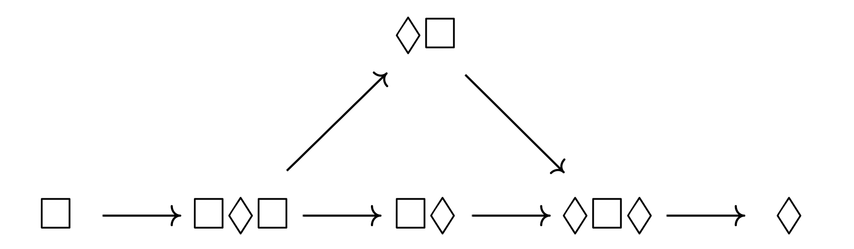
정리. S5에서 양상 연산자의 나열은 $\Box$ 또는 $\Diamond$와 동등하다. 나아가 모든 논리식은 평평한_flat 논리식 — 즉, 양상 연산자 안에 양상 연산자가 있는 경우가 없는 논리식과 동치이다.

완전성 정리

정리. K는 완전하다.

증명.

린덴바움 보조정리. 임의의 무모순적인 이론은 극대적으로 무모순적인_{maximally consistent} 이론으로 확장될 수 있다.

완전성 진술은 “무모순적인 이론은 만족 가능하다”와 동치이며, 여기에 린덴바움 보조정리를 적용하면 이는 “극대적으로 무모순적인 이론은 만족 가능하다”와 동치이다.

$u, v$가 극대적으로 무모순적인 이론이라고 하자. $\Box p \in u \implies p \in v$일 때 $u \lhd v$라고 적자. 다음을 어렵지 않게 보일 수 있다.

• $u \lhd v$일 때, $p \in v \implies \Diamond p \in u$
• 임의의 극대적으로 무모순적인 이론 $u$에 대해, $p \in u$이고 $\Box p \notin u$라면, 어떤 극대적으로 무모순적인 이론 $v, v’$가 존재하여 $p \in v, \lnot p \in v’$이고 $u \lhd v, v’$이다.

이로부터 극대적으로 무모순적인 이론 $u$에 대해, 표준적_canonical 크립키 모델 $\mathfrak{K} = (U, \prec, V)$를 다음과 같이 정의할 수 있다.

• 가능세계들의 모임 $U$는 $u \lhd v$를 만족하는 $v$의 모임이다.
• 접근 관계 $\prec$은 $\lhd$이다.
• 평가 함수_{valuation function} $V(p, v)$는 $p \in v$일 때, 그리고 오직 그 경우에만 참이다.

$\mathfrak{K}$가 $u$를 만족함을 어렵지 않게 보일 수 있다. ■

Modal Logic

01 Apr 2025

This post was originally written in Korean, and has been machine translated into English. It may contain minor errors or unnatural expressions. Proofreading will be done in the near future.

Types

Name	Entailment	Axioms
K	Kripke model for possible worlds	$\Box(p \to q) \to (\Box p \to \Box q)$
T	Reflexivity	K + $\Box p \to p$
S4	Reflexivity + Transitivity	T + $\Box p \to \Box \Box p$
S4.2	Reflexivity + Transitivity + R-convergence	S4 + $\Diamond \Box p \to \Box \Diamond p$
S4.3	Reflexivity + Transitivity + R-linearity	S4 + $(\Diamond p \land \Diamond q) \to$ $(\Diamond (p \land \Diamond q) \lor \Diamond(\Diamond p \land q))$
S5	Reflexivity + Transitivity + Symmetry	S4 + $(p \to \Box \Diamond p)$

The logics become strictly stronger as one moves down the table.

Modal Reduction

Theorem. In S4, any sequence of modal operators is equivalent to one of six combinations, and the entailment relations amongst these combinations are as follows:

Theorem. In S5, any sequence of modal operators is equivalent to either $\Box$ or $\Diamond$. Furthermore, every formula is equivalent to a flat formula—that is, a formula containing no modal operators within the scope of other modal operators.

Completeness Theorem

Theorem. K is complete.

Proof.

Lindenbaum’s Lemma. Any consistent theory can be extended to a maximally consistent theory.

The completeness statement is equivalent to “every consistent theory is satisfiable”, and applying Lindenbaum’s lemma, this is equivalent to “every maximally consistent theory is satisfiable”.

Let $u, v$ be maximally consistent theories. We write $u \lhd v$ when $\Box p \in u \implies p \in v$. The following can be shown without difficulty:

• When $u \lhd v$, we have $p \in v \implies \Diamond p \in u$
• For any maximally consistent theory $u$, if $p \in u$ and $\Box p \notin u$, then there exist maximally consistent theories $v, v’$ such that $p \in v, \lnot p \in v’$ and $u \lhd v, v’$.

From this, for a maximally consistent theory $u$, we can define the canonical Kripke model $\mathfrak{K} = (U, \prec, V)$ as follows:

• The collection of possible worlds $U$ is the collection of $v$ satisfying $u \lhd v$.
• The accessibility relation $\prec$ is $\lhd$.
• The valuation function $V(p, v)$ is true if and only if $p \in v$.

It can be shown without difficulty that $\mathfrak{K}$ satisfies $u$. ■

요네다 보조정리

21 Mar 2025

Notation.

1. $-$는 매개변수의 자릿값이다. $-$가 두 개 쓰였으면 매개변수가 두 개라는 뜻이다. 어느 매개변수가 어느 자리에 해당하는지는 맥락으로 파악한다.
2. $\bullet$은 $-$를 우선하는 매개변수이다. 따라서 $\hom(-, \bullet)$은 $A$를 함자 $\hom(-, A)$에 대응시키는 함자이다.
3. 함자 $F, G$에 대해 $[F, G]$를 $F$에서 $G$로 가는 자연적 변환_{natural transformation}들의 모임으로 정의한다.
4. 모든 범주는 국소적으로 작은_{locally small} 범주라고 가정한다.

요네다 보조정리_{Yoneda lemma}는 표현가능함자_{representable}가 다른 함자를 바라볼 때 보이는 것이 무엇인지를 알려주는 정리이다.

예를 들어 $A \in \mathcal{A}$에 대해, 표현가능함자 $\hom_{\mathcal{A}}(-, A)$를 생각하자. 이 함자가 속하는 범주는 $[\mathcal{A}^{\mathrm{op}}, \mathbf{Set}]$이다. 따라서 $\hom_{\mathcal{A}}(-, A)$가 함자 $F : \mathcal{A}^{\mathrm{op}} \to \mathbf{Set}$를 바라볼 때 보이는 것은 다음 자연적 변환들의 집합이다.

\[[\hom_{\mathcal{A}}(-, A), F]\]

위 집합은 $A \in \mathcal{A}$와 $F \in [\mathcal{A}^{\mathrm{op}}, \mathbf{Set}]$으로부터 정의된 집합이다. 그런데 $A, F$로부터 집합을 정의할 수 있는 또다른 자연스러운 방식이 있다. 단순히 $F$에 $A$를 취하는 것이다.

\[F(A)\]

요네다 보조정리에 따르면 두 집합은 동형_isomorphic이다. 게다가 그냥 동형인 것이 아니라, $A \in \mathcal{A}$와 $F \in [\mathcal{A}^{\mathrm{op}}, \mathbf{Set}]$에서 자연스럽게 동형_{naturally isomorphic}이다. 요컨대 다음 두 함자가 $[\mathcal{A}^{\mathrm{op}} \times [\mathcal{A}^{\mathrm{op}}, \mathbf{Set}], \mathbf{Set}]$에서 동형이다.

\[\begin{aligned} \text{(i)} \quad \mathcal{A}^{\mathrm{op}} \times [\mathcal{A}^{\mathrm{op}}, \mathbf{Set}] &\xrightarrow{\hspace{0.15cm} \hom_{\mathcal{A}}(-, \cdot)^{\mathrm{op}} \times 1 \hspace{0.15cm}} [\mathcal{A}^{\mathrm{op}}, \mathbf{Set}]^{\mathrm{op}} \times [\mathcal{A}^{\mathrm{op}}, \mathbf{Set}] \\ &\xrightarrow{\hom_{[\mathcal{A}^{\mathrm{op}}, \mathbf{Set}]}(-, -)} \mathbf{Set} \\\\ \text{(ii)} \quad \mathcal{A}^{\mathrm{op}} \times [\mathcal{A}^{\mathrm{op}}, \mathbf{Set}] &\xrightarrow{-(-)} \mathbf{Set} \end{aligned}\]

Remark. $\hom_{\mathcal{A}}(-, \cdot)^{\mathrm{op}}$에 붙은 $\mathrm{op}$는 함자의 정의역을 $\mathcal{A}^\mathrm{op}$로 맞춰주기 위함이고, 실질적으로는 $\hom_{\mathcal{A}}(-, \cdot)$와 같다.

증명. 증명의 개요만 적자면, $\hat{(\;\;)} : [\hom_\mathcal{A}(-, A), F] \to F(A)$와 $\tilde{(\;\;)}: F(A) \to [\hom_\mathcal{A}(-, A), F]$를 다음과 같이 정의한다.

\[\hat{\alpha} = \alpha_A(1_A), \quad \tilde{x} = \theta\]

여기서 $\theta$는 $f : A’ \to A$를 다음과 같이 사상하는 자연적 변환이다.

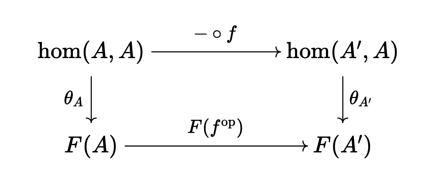
\[\theta_{A'}: f \mapsto F(f^{\mathrm{op}})(x)\]

$\theta$를 위와 같이 정의하는 이유는 다음 가환 도식을 만족하게끔 만들기 위함이다. ($(-)$에 $1_A$를 대입해 확인해 보라.)

이제 임의의 $A \in \mathcal{A}, F : \mathcal{A}^\mathrm{op} \to \mathbf{Set}$에 대해 다음이 성립함을 보여아 한다.

• 임의의 $\alpha \in [\hom_\mathcal{A}(-, A), F]$에 대해 $\tilde{\hat{\alpha}} = \alpha$이다.
• 임의의 $x \in F(A)$에 대해 $\hat{\tilde{x}} = x$이다.

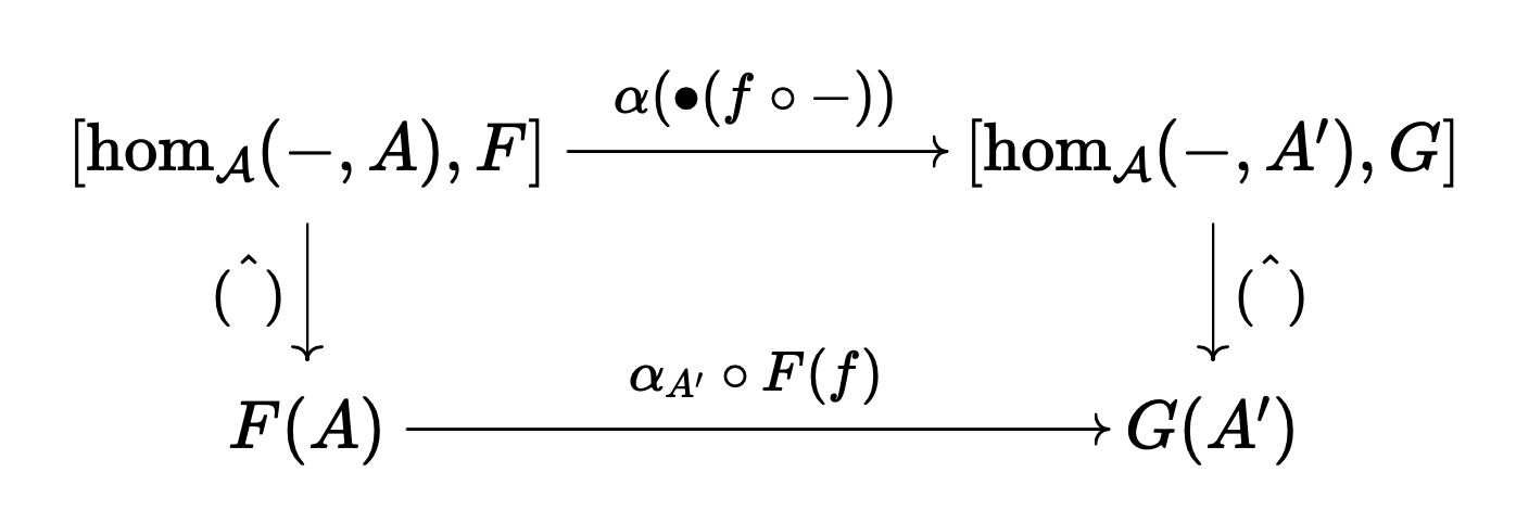
이것은 $[\hom_\mathcal{A}(-, A), F] \cong F(A)$임을 보인다. 여기에 더해, 해당 동형이 자연적임을 보여아 한다. 자아아알 생각해 보면 이것은 임의의 $A, A’ \in \mathcal{A}$와 $F, G \in [\mathcal{A}^{\mathrm{op}}, \mathbf{Set}]$와 $f: A’ \to A$와 $\alpha: F \Rightarrow G$에 대해 다음 도식이 가환임을 보이는 것과 같다.

원소 단위로 적으면,

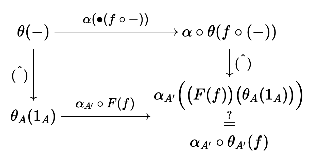
위가 성립함은 $\theta$의 자연성으로부터 따라 나온다. ■

요네다 따름정리와 관계론적 존재론

요네다 보조정리가 함의하는 결과 중 다음은 아주 중요하다. 필자는 이를 그냥 요네다 따름정리라고 부른다.

요네다 따름정리. $X, Y \in \mathcal{A}$라고 하자.

1. $[\hom(-, X), \hom(-, Y)] \cong \hom(X, Y)$
2. $X \cong Y \iff \hom(-, X) \cong \hom(-, Y)$

증명. $F = \hom(-, Y)$로 둔다. ■

요컨대 범주론에서 대상은, 그것이 받는 사상들의 집합과 다름없다. 일례로 정수 순서 범주에서 $0$은 초기 대상으로 정의할 수 있고, 더 일반적으로 $n$은 받는 사상들의 수가 $n$개인 대상으로 정의할 수 있다. 요네다 따름정리는 이처럼 대상을 그것이 다른 대상과 맺는 사상들로서 정의하는 접근이 모든(엄밀히는 국소적으로 작은) 범주에서 유효함을 보장한다. 필자는 이 접근을 관계론적 존재론이라고 부른다.

Yoneda Lemma

21 Mar 2025

This post was originally written in Korean, and has been machine translated into English. It may contain minor errors or unnatural expressions. Proofreading will be done in the near future.

Notation.

1. $-$ denotes a parameter placeholder. If two $-$ are used, it means there are two parameters. Which parameter corresponds to which position is determined by context.
2. $\bullet$ is a parameter that takes precedence over $-$. Therefore, $\hom(-, \bullet)$ is a functor that maps $A$ to the functor $\hom(-, A)$.
3. For functors $F, G$, we define $[F, G]$ as the collection of natural transformations from $F$ to $G$.
4. We assume all categories are locally small categories.

The Yoneda lemma is a theorem that tells us what a representable functor sees when it looks at another functor.

For example, for $A \in \mathcal{A}$, consider the representable functor $\hom_{\mathcal{A}}(-, A)$. This functor belongs to the category $[\mathcal{A}^{\mathrm{op}}, \mathbf{Set}]$. Therefore, what $\hom_{\mathcal{A}}(-, A)$ sees when it looks at a functor $F : \mathcal{A}^{\mathrm{op}} \to \mathbf{Set}$ is the following set of natural transformations:

\[[\hom_{\mathcal{A}}(-, A), F]\]

The above set is a set defined from $A \in \mathcal{A}$ and $F \in [\mathcal{A}^{\mathrm{op}}, \mathbf{Set}]$. However, there is another natural way to define a set from $A, F$. Simply applying $F$ to $A$:

\[F(A)\]

According to the Yoneda lemma, the two sets are isomorphic. Moreover, they are not just isomorphic, but naturally isomorphic in $A \in \mathcal{A}$ and $F \in [\mathcal{A}^{\mathrm{op}}, \mathbf{Set}]$. In short, the following two functors are isomorphic in $[\mathcal{A}^{\mathrm{op}} \times [\mathcal{A}^{\mathrm{op}}, \mathbf{Set}], \mathbf{Set}]$:

\[\begin{aligned} \text{(i)} \quad \mathcal{A}^{\mathrm{op}} \times [\mathcal{A}^{\mathrm{op}}, \mathbf{Set}] &\xrightarrow{\hspace{0.15cm} \hom_{\mathcal{A}}(-, \cdot)^{\mathrm{op}} \times 1 \hspace{0.15cm}} [\mathcal{A}^{\mathrm{op}}, \mathbf{Set}]^{\mathrm{op}} \times [\mathcal{A}^{\mathrm{op}}, \mathbf{Set}] \\ &\xrightarrow{\hom_{[\mathcal{A}^{\mathrm{op}}, \mathbf{Set}]}(-, -)} \mathbf{Set} \\\\ \text{(ii)} \quad \mathcal{A}^{\mathrm{op}} \times [\mathcal{A}^{\mathrm{op}}, \mathbf{Set}] &\xrightarrow{-(-)} \mathbf{Set} \end{aligned}\]

Remark. The $\mathrm{op}$ attached to $\hom_{\mathcal{A}}(-, \cdot)^{\mathrm{op}}$ is to adjust the domain of the functor to $\mathcal{A}^\mathrm{op}$, and is essentially the same as $\hom_{\mathcal{A}}(-, \cdot)$.

Proof. To outline the proof, we define $\hat{(\;\;)} : [\hom_\mathcal{A}(-, A), F] \to F(A)$ and $\tilde{(\;\;)}: F(A) \to [\hom_\mathcal{A}(-, A), F]$ as follows:

\[\hat{\alpha} = \alpha_A(1_A), \quad \tilde{x} = \theta\]

where $\theta$ is a natural transformation that maps $f : A’ \to A$ as follows:

\[\theta_{A'}: f \mapsto F(f^{\mathrm{op}})(x)\]

The reason for defining $\theta$ as above is to satisfy the following commutative diagram. (Verify by substituting $1_A$ for $(-)$.)

Now we must show that for any $A \in \mathcal{A}, F : \mathcal{A}^\mathrm{op} \to \mathbf{Set}$, the following holds:

• For any $\alpha \in [\hom_\mathcal{A}(-, A), F]$, we have $\tilde{\hat{\alpha}} = \alpha$.
• For any $x \in F(A)$, we have $\hat{\tilde{x}} = x$.

This shows that $[\hom_\mathcal{A}(-, A), F] \cong F(A)$. In addition, we must show that this isomorphism is natural. Upon careful consideration, this is equivalent to showing that for any $A, A’ \in \mathcal{A}$ and $F, G \in [\mathcal{A}^{\mathrm{op}}, \mathbf{Set}]$ and $f: A’ \to A$ and $\alpha: F \Rightarrow G$, the following diagram commutes:

In terms of elements:

That the above holds follows from the naturality of $\theta$. ■

The Yoneda Corollary and Relational Ontology

Among the results implied by the Yoneda lemma, the following is particularly important. I shall simply call this the Yoneda corollary.

Yoneda Corollary. Let $X, Y \in \mathcal{A}$.

1. $[\hom(-, X), \hom(-, Y)] \cong \hom(X, Y)$
2. $X \cong Y \iff \hom(-, X) \cong \hom(-, Y)$

Proof. Let $F = \hom(-, Y)$. ■

In essence, in category theory, an object is nothing more than the collection of morphisms it receives. For instance, in the integer order category, $0$ can be defined as the initial object, and more generally, $n$ can be defined as the object that receives $n$ morphisms. The Yoneda corollary guarantees that this approach of defining objects through the morphisms they form with other objects is valid in all (strictly speaking, locally small) categories. I call this approach relational ontology.

양상 문맥 내 존재 양화에 관하여 — 콰인과 프레게

18 Mar 2025

이 글은 David Kaplan, Quantifying In (1968)을 정리한 것이다.

1. 평범한 발생, 우연적 발생, 모호한 발생

다음 두 문장을 보자.

(1)과 (2)에서 모두 ‘둘’이 나타나지만, 매우 다른 방식으로 나타난다. (1)에서 ‘둘’이 나타나는 방식을 평범한 발생_{vulgar occurence}이라고 하고, (2)에서 ‘둘’이 나타나는 방식을 우연적 발생_{accidental occurence}이라고 하자.

단어가 평범하게 발생할 경우 해당 단어는 지시하며, 동일성에 대한 라이프니츠 원리를 만족한다(예컨데 ‘둘’을 ‘화성의 위성 개수’로 대치해도 문장의 진릿값이 보존된다). 단어가 우연적으로 발생할 경우 해당 단어는 지시하지 않으며, 라이프니츠 원리를 만족하지 않는다.

이제 다음의 문장들을 보자.

(3), (4), (5)에서 ‘둘’은 지시를 하는 것으로 보인다. 그러나 ‘둘’을 ‘화성의 위성 개수’로 바꾸면 문장의 진릿값이 보존되지 않는 것으로 보인다. 이것을 모호한 발생_{intermediate occurence}이라고 하자.

언어철학에서 모호한 발생은 크게 두 가지 방식으로 설명된다. 첫째는 모호한 발생을 우연적 발생에 동화하는 것이고, 둘째는 모호한 발생을 평범한 발생에 동화하는 것이다.

2. 콰인: 모호한 발생은 우연적 발생이다

콰인은 모호한 발생을 우연적 발생에 동화한다. 그는 (3)에서 따옴표로 감싸진 문장은 하나의 단어이고, (5)에서 둘이 하나보다 크다고 믿었다 는 원자 술어라고 주장한다. 특히 (3), (4), (5)에서 ‘둘’이 나타나는 문맥을 불투명 문맥_{opaque context}이라고 명명한 것은 그가 모호한 발생과 우연적 발생의 동일시를 염두에 뒀음을 시사한다.

콰인은 (3), (4), (5)와, 다음의 (6), (7), (8)을 대조한다.

(3), (4), (5)와 달리 (6), (7), (8)의 문형에서 ‘둘’은 평범하게 발생하는 것으로 보인다 (콰인이라면 ‘하나’는 여전히 우연적으로 발생한다고 주장할 것이다). 그러나 (6), (7), (8)은 고전 논리로 표현할 수 있는 문장이 아니다. 고전 논리는 ‘There exists $x$ such that…‘이라는 문형은 허용하지만 ‘$n$ is such that…‘이라는 표현은 결여하기 때문이다. 따라서 (6), (7), (8)의 의미론을 정당화하는 것이 과제로 남는다.

우선 (6)부터 보자. 최소한의 논리적 분석으로도 (6)이 적형식_{well-formed formula}이 아님을 알 수 있다. 주어의 둘 은 이름의 사용_use에 해당하지만, 뒤에 ‘하나보다 크다’를 적기 는 이름의 언급_mention에 해당하기 때문이다. 따라서 (6)은 의미론적으로 정당하지 않다.

(7)의 의미는 아리스토텔레스적 본질주의_{Aristotelian essentialism}로써 설명할 수 있다. 이 설명은 임의의 대상에 대해, 그에게 본질적인 속성과 우연적인 속성이 무엇인지를 규정한다. 콰인은 이같은 방식으로 (7)의 정당성을 설명한 바 있다.

(8)이 의미론적으로 정당함을 시사하는 예시는 많이 있다. 러셀의 다음 유명한 문장을 보자.

• 네 요트의 길이에 대해, 내가 생각한 네 요트의 길이는 그것보다 길다. _{The length of your yacht is such that I thought that your yacht was longer than that.}

위 문장은 직관적으로 이해가 되며, 참인 듯하다. 이것은 (8)의 의미론적 정당성을 지지한다. 또한 콰인은 다음의 유명한 문장의 쌍을 거론한다.

a. 랄프는 누군가가 스파이라고 믿는다. _{Ralph believes that someone is a spy.}

b. 누군가에 대해, 랄프는 그가 스파이라고 믿는다. _{Someone is such that Ralph believes they are a spy.}

a에서는 존재 양화가 믿음 문맥 안에서, b에서는 밖에서 이루어진다. 한편 콰인은 믿음 문맥 속의 단어들을 우연적 발생과 동일시하기 때문에, 그에 따르면

• 랄프는 올트커트가 스파이라고 믿는다.

로부터 $\exists$-첨가를 적용하여 b를 유도할 수 없음에 유의하라. 그러나,

• 올트커트 씨에 대해, 랄프는 그가 스파이라고 믿는다.

로부터 b를 유도하는 것은 가능하다.

결론적으로 애매한 발생에 대한 콰인의 입장은 두 가지이다. 첫째, 애매한 발생은 우연적 발생과 동일시할 수 있다. 둘째, 불투명 문맥 안과 밖에서 단어가 등장하는 경우를 구분해야 할 필요가 있을 때는 ‘…에 대해_{such that}’ 구문을 사용할 수 있다. 콰인은 이 구문을 관계론적 의미에서의 믿음_{relational sense of belief}이라고 부른다. 마찬가지로 우리는 관계론적 의미에서의 양상, 주장, 생각 등의 구문을 도입할 수 있겠으나, 각 구문의 도입은 별도의 정당화를 요구한다.

3. 프레게: 모호한 발생은 평범한 발생이다

프레게는 모호한 발생을 평범한 발생에 동화한다. 프레게는 모호한 발생에서 라이프니츠 원리가 어긋나는 것으로 보이는 이유는, 해당 문맥에서 단어들의 실제 지시체를 우리가 혼동하기 때문이라고 주장한다. 이 혼동에는 두 가지 원인이 있다. 첫째는 지시 표현이 언제나 동일한 대상을 지시한다는 믿음이다. 이로부터 도출되는 둘째 믿음은, 대부분의 맥락에서 같은 대상을 지시하는 지시 표현은 언제나 같은 대상을 지시한다는 믿음이다.

그러나 지시 표현이 언제나 같은 대상을 지시한다는 믿음에 반하는 사례는 많다. 일례로 다음과 같이 중의적이거나 모호한_ambiguous 단어의 사례가 있다.

(11)에 대한 자연스러운 분석은, 전자의 ‘F.D.R.’은 정치인을 지칭하는 한편 후자의 ‘F.D.R.’은 텔레비전 방송을 지칭한다고 보는 것이다. 이 경우 두 ‘F.D.R.’은 모두 평범한 발생이다. 그러나 극단적인 이름-지시체-일대일-대응-주의자라면 (11)이 ‘텔레비전에 딱 한 번 방영되었다’가 불투명 문맥임을 드러내며, 후자의 ‘F.D.R.’은 우연적 발생이라고 주장할지 모른다. 이 입장을 조금 더 그럴듯하게 포장하면, (11)은 올바르지 않은 문장이며 후자의 ‘F.D.R.’은 ‘‘F.D.R’이라는 이름의 텔레비전 방송’으로 수정되어야 한다고 주장할 수 있다.

이 사례가 보여주는 것은, 누군가 불투명 문맥으로 이해할 문장을 누군가는 모호함의 발생으로 이해할 수 있다는 것이다. 프레게는 지시 표현은 보통 그 일상적인 지시체를 지시하지만, 뜻_sense 따위의 중간 대상을 지시할 수도 있으며, 이같은 모호함이 철학자들을 애매한 발생의 문제로 빠뜨린 원인이라고 주장한다. 프레게는 전자를 직접 지시_{direct reference}, 후자를 간접 지시_{indirect reference}라고 부른다.

	콰인	프레게
둘은 하나보다 크다	지시 문맥	직접 지시
필연적으로, 둘은 하나보다 크다	불투명 문맥	간접 지시

그렇다면 애매한 발생에서 표현의 지시체가 무엇인지 어떻게 알아낼 수 있을까? 저자는 합성의 원리_{principle of compositionality}가 핵심이라고 말한다. 문장을 이루는 개별 요소의 지칭체가 불분명하다면, 문장 전체의 지칭체를 먼저 확인하고, 문장의 지칭체가 어떻게 분석 가능한지를 파악함으로써 개별 요소의 지칭체를 역추적할 수 있다는 것이다.

이 방법론에 따라 프레게는 인용구 안의 표현_expression들은 자기 자신을 지시한다는 입장에 도달했다. 예를 들어 $\ulcorner 1 + 2 = 3 \urcorner$에서 $\ulcorner 1 \urcorner$의 지시체는 $\ulcorner 1 \urcorner$이다. 이같은 프레게의 입장은 인용 문맥 내의 양화사 사용을 가능하게 만든다. 로마 문자의 정의역이 대상이고, 그리스 문자의 정의역이 표현이라고 하면 프레게의 이론 하에서 우리는 다음과 같은 참을 표현할 수 있다.

표현에 비해 뜻_sense 또는 의미_meaning의 존재론적 위상은 불분명하지만, 비슷한 접근을 시도해 볼 수 있다. 먼저 다음의 사례로 예증되는 의미 따옴표를 도입하자.

고딕 문자의 정의역이 의미라고 하면 프레게주의는 다음과 같은 참을 표현할 수 있다.

Remark. 작은따옴표는 표현을 나타내는 반면, $\ulcorner$…$\urcorner$은 표현들의 합성을 의미한다. 마찬가지로 ^m…^m은 의미를 나타내는 반면, ^M…^M은 의미들의 합성을 의미한다. 물론 표현들의 합성도 표현이고, 의미들의 합성도 의미이기 때문에, 등식 1, 2가 성립한다. 저자가 등식 1, 2를 등식 3에 빗대어 설명했다는 사실을 떠올리면 도움이 된다.

1. ‘The cat is on the mat’ $=$ $\ulcorner$The cat is on the mat$\urcorner$
2. ^mThe cat is on the mat^m $=$ ^MThe cat is on the mat^M
3. $237 = 2 \times 10^2 + 3 \times 10 + 7$

그러나 작은따옴표와 $\ulcorner$…$\urcorner$가 완전히 같고, 그리고 ^m…^m과 ^M…^M이 완전히 같은 것은 결코 아니다. 각 경우 전자는 불투명하지만 후자는 투명하기 때문이다. 따라서 1은 불가능하지만 2는 가능하다. 이것은 3은 말이 안 되지만 4는 올바른 것과 같은 이치이다.

1. $\exists \alpha\; \big($ ‘$\alpha$ is on the mat’ is true$\big)$
2. $\exists \alpha\; \big(\ulcorner \alpha$ is on the mat$\urcorner$ is true$\big)$
3. $\exists n\; (237 < 2n7)$
4. $\exists n\; (237 < 2 \times 10^2 + n \times 10 + 7)$

4. 지시 술어를 통한 프레게주의의 보강

이제 프레게주의가 (6), (7), (8)을 어떻게 설명하는지 보자.

그에 앞서, (4), (5), (7), (8)에서 믿음의 대상이 되는 것이 정확히 무엇인지를 명료화하는 것이 도움이 된다. S가 문장일 때, 누군가가 S를 믿는다는 것, 또는 S가 필연적이라는 것은 어떻게 형식화할 수 있는가? 본 논문에서는 간단한 길을 택하여, 문장은 자기 자신을 지시하는 것으로 간주하고, 필연을 문장에 대한 단항 술어로, 믿음을 주체와 문장 사이의 이항 술어로 간주한다. 따라서 (4), (5)는 다음과 같이 적을 수 있다.

(7), (8)을 콰인식으로 형식화하기 위해, 콰인의 관계론적 믿음과 관계론적 필연을 나타낼 술어 $\mathbf{Nec}$와 $\mathbf{Bel}$를 도입하자.

여기서 볼드체 문자 $\mathbf{x}$는 $\mathbf{x}$가 지시적으로서가 아닌, 오직 자리값_placeholder으로서 사용되었음을 의미한다. 콰인에 따르면 $\mathbf{x}$는 불투명 문맥에 있으므로, 지시할 수 없기 때문이다.

프레게주의는 (15)와 (16)을 다음과 같이 형식한다.

상술한 Remark로 인해 동일한 술어 $\mathbf{N}, \mathbf{B}$를 사용할 수 있다.

하지만 (19)와 (20)만으로는 부족한 점이 있다. (19)와 (20)의 ‘둘’이 지시적이긴 하지만, (7)과 (8)의 ‘둘’과는 다른 대상을 지시한다. 전자는 표현을, 후자는 수를 지시하기 때문이다. 따라서 (7)과 (8), 또는 (17)과 (18)로부터 가능했을 논리적 추론이 (19)와 (20)만으로는 얻어지지 않는다. 예를 들어 (17)과 다음이 주어졌을 때,

다음을 도출할 수 있다.

그러나 (19)와 (21)은 다음을 도출하는 데 그친다.

• $\exists y \big(y =$ 화성의 위성 수 $\land$ $\mathbf{N}\ulcorner$둘은 하나보다 크다$\urcorner\big)$

한편 다음은 올바르지 않다. $\alpha$는 수가 아니라 표현이기 때문이다.

• $\exists \alpha \big(\alpha =$ 화성의 위성 수 $\land$ $\mathbf{N}\ulcorner \alpha$는 하나보다 크다$\urcorner\big)$

그러나 이 문제는 처치가 도입한 바 있는 지시 술어 $\Delta$를 도입함으로써 해결할 수 있다. $\alpha$가 $c$를 지칭할 때, 그리고 오직 그럴 때만 $\Delta(\alpha, c)$라고 하자. 그러면 프레게식으로 (22), (17), 그리고 (18)은 각각 다음과 같이 적을 수 있다.

논문의 저자는 (23), (24), (25)가 원 문장의 직관적인 의미를 포착할 뿐 아니라, 콰인과 달리 $\mathbf{Bel}, \mathbf{Nec}$ 등의 추가적인 술어를 소개하고 정의할 필요가 없다는 점을 강조한다.

5. 올트커트 역설

콰인은 다음의 사고실험을 제시한 바 있다. 랄프는 골목에서 갈색 모자를 쓴 수상한 인물이 벤치 밑의 서류가방을 가져가는 것을 보고는 그가 스파이일 것이라고 믿는다. 한편 랄프는 그가 속한 도시의 시장을 존경하며, 그가 스파이일 리가 없다고 믿는다. 그런데 사실 수상한 사람과 시장은 동일한 인물, 올트커트 씨이다.

콰인은 이를 다음과 같이 형식화한다.

(26), (27)을 관계론적 믿음으로 표현하면,

(28)에 의해 (29), (30)은 각각 다음을 시사한다.

따라서 랄프는 다음을 믿는 것으로 보인다.

그러나 (34)는 문제적이다. 콰인은 문제의 원인이 (32), (33)으로부터 (34)를 도출하는 데 있다고 주장한다. 프레게적 형식화는 콰인의 직관이 올바름을 증명한다. 자세한 과정은 생략하지만, (26), (27), (28)은 오직 다음을 도출한다.

여기까지는 좋다. 문제는 두 번째 역설이다. (9)가 참이라고 하자. 즉, 랄프는 스파이의 존재를 믿는다. 또한 랄프는 세상에 키가 정확히 똑같은 두 사람은 존재하지 않는다고 믿으므로 (매우 합당한 믿음이다) 키가 가장 짧은 스파이가 존재하리라 믿는다. 따라서 (39)가 성립한다.

콰인식으로 ‘키가 가장 작은 스파이’를 추출_exportation하면,

$\exists$-첨가에 의해,

그리고 (41)은 (10)과 내용이 같다. 따라서 (9)와 (10)이 서로를 시사하게 되는 모순이 발생한다. 논문의 저자는 이 문제가 너무 까다로운 나머지 한때 양상 및 믿음 문맥에서 양화하는 것은 불가능하다는 입장으로 기울었으나, 이를 공략할 방안이 떠올랐다는 일화를 이야기한다. 이에 대해서는 다음 글에서 소개하도록 하겠다.