On Reference — Descriptivism and Causal Theory

07 Jan 2025

This post was originally written in Korean, and has been machine translated into English. It may contain minor errors or unnatural expressions. Proofreading will be done in the near future.

This article is a summary and analysis of the Stanford Encyclopedia of Philosophy entry on reference.

1. Introduction

In “That is Venus” and “The last Queen of England is Elizabeth II”, the expressions ‘that’, ‘Venus’, ‘the last Queen of England’, and ‘Elizabeth II’ are expressions that refer to exactly one object in this world by specifying it. However, the specific principles by which these expressions come to refer to particular objects are shrouded with philosophical puzzles.

This article addresses six questions:

1. The subject of referring: Is reference done by the speaker via their intention, or by the word via its meaning?
2. The meaning of referring expressions: Is it a (defininte) description, the referent, or something else?
3. The mechanism of reference: What grounds the correspondence between referring expressions and referred objects?
4. The scope of theories of reference: Do all referring expressions share a common mechanism?
5. The privacy of reference: To what extent does reference depend on the speaker’s private states (e.g. intentions to refer)?
6. The significance of theories of reference: Does the reference relation actually exist? Is it philosophically significant?

This article examines four theories: descriptivism, causal theory, character model, and intentionalism, and briefly discusses referential scepticism.

	Descriptivism	Causal Theory	Character Model	Intentionalism
Subject	Speaker	Referring expression	Pluralistic	Speaker
Meaning	Descriptive content	Referent	Character and content
Mechanism	Words are associated with specific descriptive content and refer to objects that satisfy them.	Words are associated with causal chains that trace back to the referent’s initial baptism.	Words are associated with conventional referential rules (character) to refer its referent (content).	Words are epiphenomenal to the speaker’s intention to refer to a specific objects.
Scope	Broad	Narrow (names)	Moderate	Broad
Privacy	Strong privacy	Weak privacy	Moderate privacy	Strong~moderate privacy
Scholars	(Frege), Russell, Strawson, Reichenbach	Mill, Kripke, Kaplan	Kaplan	Kaplan, Grice, Reimer
Strengths	Solves Frege’s puzzle	Solves Kripke’s arguments	Explains how pure indexicals work	Explains how impure indexicals work
Weaknesses	Kripke’s modal and semantic arguments	Problems with names having multiple bearers	Speaker-hearer dilemma arises with impure indexicals	Humpty Dumpty problem

2. Proper Names

2.1. Descriptivist Theory of Proper Names

Descriptivist Thesis.

1. A proper name $n$ is associated with specific descriptive content $P$.
2. $n$ is associated with $P$ because the speaker privately (mentally) associates $n$ with $P$.
3. When there exists a unique object $c$ that satisfies $P$, $n$ refers to $c$.
4. The meaning of $n$ ($P$) and the referent of $n$ ($c$) are distinct, with the former determining the latter.

For example, a speaker who associates the name ‘Venus’ with the descriptive content “the second planet of the solar system” refers to Venus using ‘Venus’ because there is a unique object satisfying that descriptive content, and that object is Venus.

Remark.

1. while it is standard to understand descriptive content as descriptions, scholars such as Searle argue that descriptive content need not be linguistically specifiable but may also be based on perception.

2. The satisfaction relation of descriptive content is speaker-independent. As we shall see, this spells problem in explaining indexicals.

3. Furthermore, the satisfaction relation is de dicto. As we shall see, this spells problem in dealing with modality.

4. Theses 1, 3, 4 provide a semantics for names — a theory specifing the domain (names) and codomain (descriptive content) of the meaning function $M$ — while thesis 2 provides a metasemantics for names — a theory explaining how the map $n \mapsto M(n)$ is defined for each name $n$.

Argument 1. Cases of Names with Multiple Bearers

Consider a case where A and B know two people named ‘Boris Johnson’. One is a colleague of A and B, and the other is the former Prime Minister of Britain. When A says to B, “Boris Johnson has made a grave mistake,” B asks, “Which Boris Johnson do you mean?” To this, A replies, “The former Prime Minister of Britain.”

In the above case, it appears that (1) the speaker A has the authority to determine what ‘Boris Johnson’ refers to, and this determination is made (2) via the descriptive content that the speaker has in mind.

Argument 2. Frege’s Puzzle

Consider the following examples:

1. The morning star is the evening star.
2. Santa Claus lives at the North Pole.
3. Fred believes that Mark Twain was American but does not believe that Samuel Clemens was American.

Let us first make some remarks. Statement 1 is true but not a priori. Statement 2 is not incomprehensible. Fred’s belief expressed in Statement 3 is not inconsistent.

If the meaning of a name were its referent, then 1 would be a priori by the law of self-identity, 2 would be nonsense as it has as its subject an expression lacking a referent, and in case 3, Fred’s belief would be inconsistent since Mark Twain and Samuel Clemens share the same referent. On the other hand, descriptivism provides adequate explanations for all three statements by distinguishing between the meaning and referent of names.

Objection 1. The Modal Argument

Even if I associate the description “the former British Prime Minister who implemented Brexit” with ‘Boris Johnson’, I can still assert the following sentence as true:

1. Boris Johnson might not have implemented Brexit.

However, if the meaning of a name is equivalent to a description, then 1 is equivalent to 2.

2. The following might have been the case: the former British Prime Minister who implemented Brexit did not implement Brexit.

But 2 is false. Therefore, the meaning of a name is not descriptive content.

Remark. Since the meaning of the name is de dicto, the inference from 1 to 2 is a de dicto substitution. In the case of de re substitution, 1 becomes 3.

3. Let $c$ be that person who is the former British Prime Minister who implemented Brexit. Then the following might have been the case: $c$ did not implement Brexit.

Unlike 2, there is no problem in regarding 3 as true. Hence, to deal with the modal argument, descriptivists may attempt to modify theses 3 and 4.

1. When there exists a unique object $c$ that satisfies $P$ in the actual world, $n$ refers to $c$.

2. The meaning of $n$ is the referent of $n$, i.e., $c$. (That is, the meaning of $n$ is de re)

However, this modified descriptivism not only fails to adequately explain Frege’s puzzle but also fails to adequately explain the following semantic argument, making it a theory with many limitations.

Objection 2. The Semantic Argument

The semantic argument is an argument that refutes a group of theories belonging to descriptivism, including the modified descriptivism just presented. The gist is that in many cases, the descriptive content $P$ that a speaker associates with a name $n$ fails to uniquely pick out a specific object in the world (i.e., the description is insufficient), and descriptive content is unnecessary for reference in the first place.

As a case showing that descriptive content is insufficient, there is the Feynman-Gell-Mann thought experiment presented by Kripke. The descriptive content that most people associate with the name ‘Feynman’ is something like “a famous American physicist”. This description also applies to Gell-Mann. However, we seem to successfully refer to Feynman with the name ‘Feynman’.

Furthermore, as a case showing that descriptive content is unnecessary, consider the Gödel-Schmidt thought experiment likewise presented by Kripke. Kripke assumes the following situation:

In fact, the mathematician who first proved the incompleteness of arithmetic was not Gödel but an unknown mathematician named Schmidt. However, before publishing the proof, Schmidt died under mysterious circumstances, and his proof fell into Gödel’s hands and was published under Gödel’s name.

(Regarding this bizarre thought experiment, there is a rumour that it was Kripke’s way of venting his jealousy towards Gödel, a logician greater than himself)

If (P1) the above assumption is true, (P2) descriptivism is correct, and (P3) the descriptive content that most people associate with the name ‘Gödel’ is “the mathematician who first proved the incompleteness of arithmetic”, then (C) the object that most people refer to with the name ‘Gödel’ is Schmidt, not Gödel. However, this is counterintuitive. Therefore, descriptivism is not correct.

Remark. To overcome the semantic argument, descriptivists can take one of two approaches:

1. The descriptive content associated with a name can transcend information personally available to the speaker.

2. The descriptive content associated with a name can adopt “the person whom the person who transmitted this name to me intended to refer to with that name”.

Strawson chooses approach 1. According to him, speakers can rely on others for the task of providing the descriptive content that should be associated with names. In this case, the meaning of ‘Feynman’ or ‘Gödel’ is the descriptive content that Feynman experts or Gödel experts associate with each name. However, Strawsonian theory has the limitation of being counterintuitive in that it makes the speaker’s referential intention irrelevant to the actual reference.

Approach 2 is closely connected to causal theory. Let us examine this theory.

2.2. Millianism and Causal Theory of Proper Names

Millian Thesis. The meaning of a proper name is its referent.

As the name suggests, this position traces back to John Stuart Mill. Millian theories imply that identity statements such as “The morning star is the evening star” are a posteriori but necessarily true.

Remark. Kripke also argues that there exist sentences that are a priori but contingently true, citing “The length of the standard metre is 1m” as an example.

The Millian thesis provides semantics for names. A representative metasemantics supplementing this is the causal theory.

Causal Theory.

1. There is an initial baptism, an event in which object $c$ is first called by name $n$.
2. Starting with those who participated in the initial baptism, speakers who refer to $c$ with $n$ transmit this usage to other speakers through communication. Such transmission of usage forms a causal chain of the name.
3. The meaning (referent) of name $n$ is the object named in the initial baptism that occurred at the starting point of $n$’s causal chain.

One subtle problem with causal theory is distinguishing which communicative transmissions substantially participate in the causal chain. For instance, if I called my arrogant cat ‘Napoleon’ to a work colleague, this communication does not substantially participate in the causal chain of the name ‘Napoleon’ (parasitic use of names). There are also cases where the referent of a name changes along the way, such as the Madagascar case (confused use of names). We omit discussion of this problem here.

2.3. The Problem of Names with Multiple Bearers

In cases of names with multiple bearers, such as the earlier ‘Boris Johnson’ example, the authority to determine reference seems to lie with the speaker. This fact poses no problem for classical descriptivism. However, this

In cases of names with multiple bearers, such as the earlier ‘Boris Johnson’ example, the authority to determine reference seems to lie with the speaker. This fact poses no problem for classical descriptivism. However, this spells trouble for Strawsonian and causal theories.

In the case of Strawson’s theory, the referent of a name $n$ is uniquely determined by a group of experts, so it can have at most one referent. However, since names with multiple bearers are clearly possible, Strawson’s theory must consider names in a more nuanced way. That is, it must acknowledge the possibility of names that are literally equivalent ($\ulcorner n_1 \urcorner = \ulcorner n_2 \urcorner$) but semantically different ($n_1 \mapsto c_1, n_2 \mapsto c_2, c_1 \neq c_2$). However, this raises the question of what principle determines $i$ when the speaker utters $\ulcorner n_i \urcorner$. This principle cannot be the speaker’s internal description, as one can imagine a speaker who can refer to either $c_1$ or $c_2$ using $\ulcorner n_i \urcorner$, but lacks sufficient descriptive content to distinguish between $c_1$ and $c_2$.

I cannot accept the italicised content. Are there really such cases?

A similar problem arises in Millianism. To overcome this issue, Kaplan considers names as psychological phenomena. That is, a name $n$ is a psychological phenomenon intertwined with the literal content $\ulcorner n \urcorner$ and the intention to refer to $c$ using $\ulcorner n \urcorner$, and what is transmitted through the causal chain is this psychological phenomenon. According to this view, names with multiple bearers are distinguished as $n_1 = (\ulcorner n \urcorner, c_1), n_2 = (\ulcorner n \urcorner, c_2)$, and a speaker who has successfully acquired $n_1$ and $n_2$ can choose to use either $n_1$ or $n_2$ according to their intention.

Another approach that differs from Kaplan’s is the attempt to resolve the problem of multiple bearers through a combination of causal theory and indexical theory. This approach has been adopted by Lucanati, Pelcher, and Rainsbury, and requires an understanding of the indexical theory that will be examined in the following text.

대각선 논법 없이 실수의 비가산성 증명하기

26 Dec 2024

정리. $\mathbb{R}$은 비가산이다. 즉, $\mathbb{N}$에서 $\mathbb{R}$로 가는 전사함수는 존재하지 않는다.

수학과 2학년 정도 되면 한번쯤은 들어 봤을 정리이다. 가장 널리 알려진 증명은 칸토어의 대각선 논법이다. 하지만 대각선 논법 없이 이 정리를 증명하는 방법이 있다. 각각 $\mathbb{R}$의 순서적 특징과, 위상적 특징을 이용한다.

1. 동형성 정리를 이용한 증명

칸토어의 동형성 정리에 따르면 다음을 만족하는 전순서 집합 $(S, \leq)$는 모두 순서 동형이다.

1. $S$는 가산이다.
2. $S$는 조밀하다. 즉, $x, y \in S$에 대해 $x < y$라면 $x < z < y$인 $z \in S$가 존재한다.
3. $S$는 상계 및 하계를 가지지 않는다.

$(\mathbb{Q}, \leq)$는 위 세 조건을 모두 만족하고, $(\mathbb{R}, \leq)$는 2와 3을 만족한다. 따라서 만약 $\mathbb{R}$이 가산이면 $(\mathbb{R}, \leq)$는 $(\mathbb{Q}, \leq)$와 순서 동형이다. 하지만 전자는 완비인데 반해 후자는 그렇지 않으므로 $\mathbb{R}$은 비가산이다. ■

2. 콤팩트성을 이용한 증명

$X$가 고립점이 없는 콤팩트한 하우스도르프 공간이라고 하자. 또한 $X \neq \varnothing$이라고 하자.

Claim 1. $U \neq \varnothing$가 $X$의 열린 집합이라고 하자. $x \in X$에 대해 $x \notin \bar{V}$이면서 $V \subset U$인 열린 집합 $V$가 존재한다.

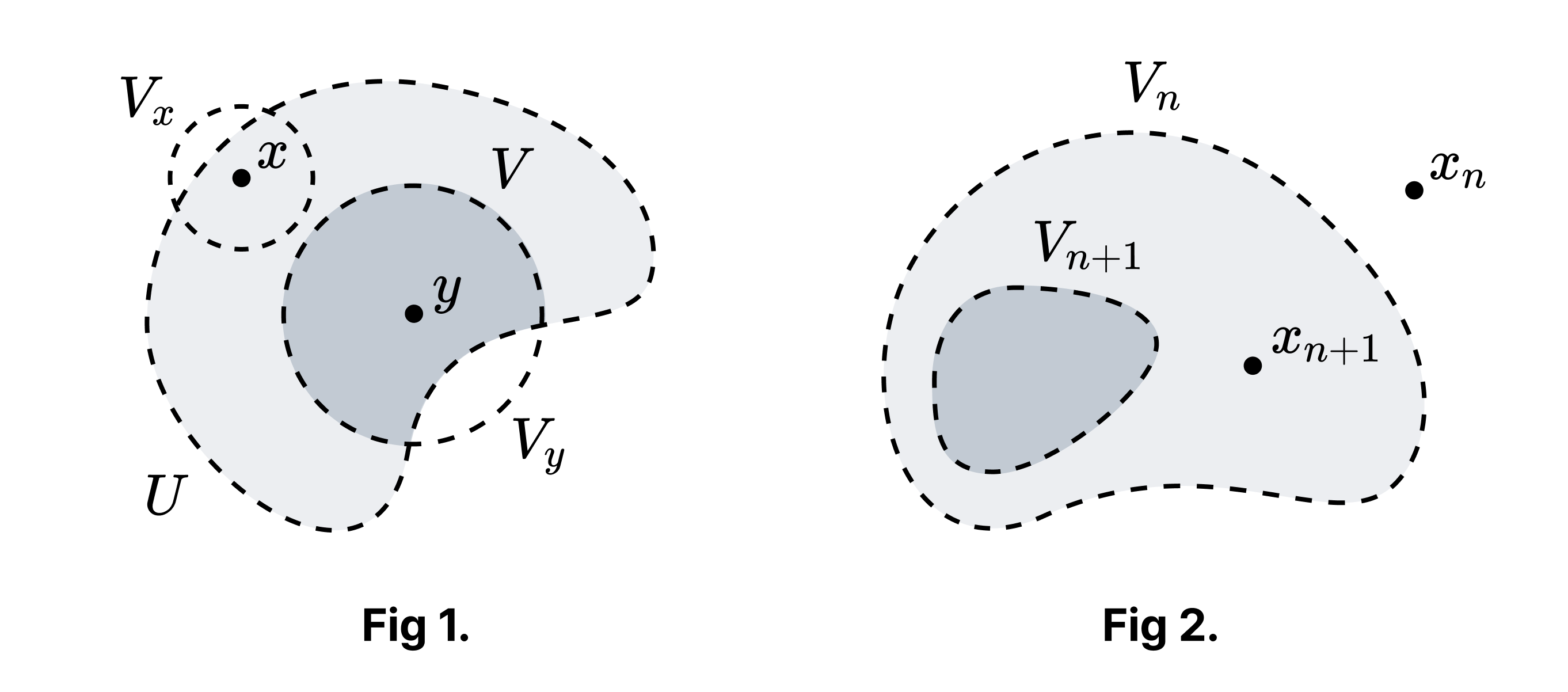
Proof of Claim 1. $x \neq y$이며 $y \in U$가 존재한다. 왜냐하면 $x \in U$인 경우 $X$가 고립점을 가지지 않으므로 존재하고, $x \notin U$인 경우 $U$가 공집합이 아니기 때문에 존재하기 때문이다. $X$가 하우스도르프이므로 $x, y$를 근방 $V_x, V_y$로 분리할 수 있다. $V = V_y \cap U$가 얻고자 하는 집합이다 (Fig 1에서 짙게 색칠된 영역). □

Claim 2. $X$는 비가산이다.

Proof of Claim 2. $X$가 가산이라고 하자. $X$의 원소들을 $\lbrace x_n \rbrace_{n \in \mathbb{Z}^+}$와 같이 나열한다. $V_0 = X$라고 하자. Claim 1에 의해 각 $n$에 대해 $x_n \notin \bar{V_n}$인 열린 집합 $V_n$이고 $V_n \subset V_{n-1}$인 열린 집합 $V_n$이 존재한다 (Fig 2). $X$가 콤팩트하므로 유한 교집합 성질에 의해

\[K = \bigcap_{n \in \mathbb{Z}^+} \bar{V}_n \neq \varnothing\]

이다. 하지만 $x_n \in K$라면 $x_n \in \bar{V}_n$이 되어 모순이다. 따라서 $X$는 비가산이다. □

Claim 3. $\mathbb{R}$은 비가산이다.

Proof of Claim 3. $[0, 1]$은 고립점을 가지지 않는 콤팩트 하우스도르프 공간이다. 따라서 비가산이다. 이에 따라 $\mathbb{R}$은 비가산이다. ■

Proving the Uncountability of Real Numbers Without the Diagonal Argument

26 Dec 2024

Theorem. $\mathbb{R}$ is uncountable. That is, there exists no surjective function from $\mathbb{N}$ to $\mathbb{R}$.

This is a theorem that any sophomore student would have encountered at least once. The most widely known proof is Cantor’s diagonal argument. However, there are methods to prove this theorem without the diagonal argument. These utilise the order-theoretic and topological properties of $\mathbb{R}$, respectively.

1. Proof Using the Isomorphism Theorem

Cantor’s isomorphism theorem states that all totally ordered sets $(S, \leq)$ satisfying the following conditions are order isomorphic:

1. $S$ is countable.
2. $S$ is dense. That is, for $x, y \in S$ with $x < y$, there exists $z \in S$ such that $x < z < y$.
3. $S$ has neither an upper bound nor a lower bound.

$(\mathbb{Q}, \leq)$ satisfies all three conditions above, while $(\mathbb{R}, \leq)$ satisfies conditions 2 and 3. Therefore, if $\mathbb{R}$ were countable, then $(\mathbb{R}, \leq)$ would be order isomorphic to $(\mathbb{Q}, \leq)$. However, the former is complete while the latter is not, so $\mathbb{R}$ is uncountable. ■

2. Proof Using Compactness

Let $X$ be a compact Hausdorff space with no isolated points. Also assume that $X \neq \varnothing$.

Claim 1. Let $U \neq \varnothing$ be an open subset of $X$. For $x \in X$, there exists an open set $V$ such that $x \notin \bar{V}$ and $V \subset U$.

Proof of Claim 1. There exists $y \in U$ where $x \neq y$. This is because if $x \in U$, then since $X$ has no isolated points such a $y$ must exist, and if $x \notin U$, then such a $y$ exists because $U$ is non-empty. Since $X$ is Hausdorff, we can separate $x$ and $y$ by neighbourhoods $V_x$ and $V_y$. Then $V = V_y \cap U$ is the desired set (the dark shaded region in Fig 1). □

Claim 2. $X$ is uncountable.

Proof of Claim 2. Suppose $X$ is countable. Enumerate the elements of $X$ as $\lbrace x_n\rbrace _{n \in \mathbb{Z}^+}$. Let $V_0 = X$. By Claim 1, for each $n$ there exists an open set $V_n$ such that $x_n \notin \bar{V_n}$ and $V_n \subset V_{n-1}$ (Fig 2). Since $X$ is compact, by the finite intersection property we have

\[K = \bigcap_{n \in \mathbb{Z}^+} \bar{V}_n \neq \varnothing.\]

However, if $x_n \in K$, then $x_n \in \bar{V}_n$, which is a contradiction. Therefore, $X$ is uncountable. □

Claim 3. $\mathbb{R}$ is uncountable.

Proof of Claim 3. $[0, 1]$ is a compact Hausdorff space with no isolated points. Therefore, it is uncountable. Consequently, $\mathbb{R}$ is uncountable. ■

칸토어-벤딕슨 정리와 폴란드 공간

25 Dec 2024

정의. 위상공간 $X$의 집합 $P$에 대해 $P’ = P$일 때 $P$를 완벽한 집합_{perfect set}이라고 한다. ($P’$은 $P$의 집적점들의 집합)

Remark. 모든 완벽한 집합은 닫힌 집합이지만, 역은 성립하지 않는다. 일반적으로 $S \not\subset S’$ ($S$가 고립점을 가짐), $S’ \not\subset S$ ($S$가 닫힌 집합이 아님) 임에 유의하라. 뒤집어 말해, 완벽한 집합은 고립점이 없는 닫힌 집합이다.

정의. $X$의 임의의 부분공간이 린델뢰프일 때 $X$를 세습적 린델뢰프_{hereditarily Lindelöf}라고 한다.

약한 칸토어-벤딕슨 정리. $X$가 세습적 린델뢰프 공간이라고 하자. $F \subset X$가 닫힌 집합일 때 어떤 완벽한 집합 $P$와 가산집합 $C$가 존재하여 $F = P \sqcup C$이다.

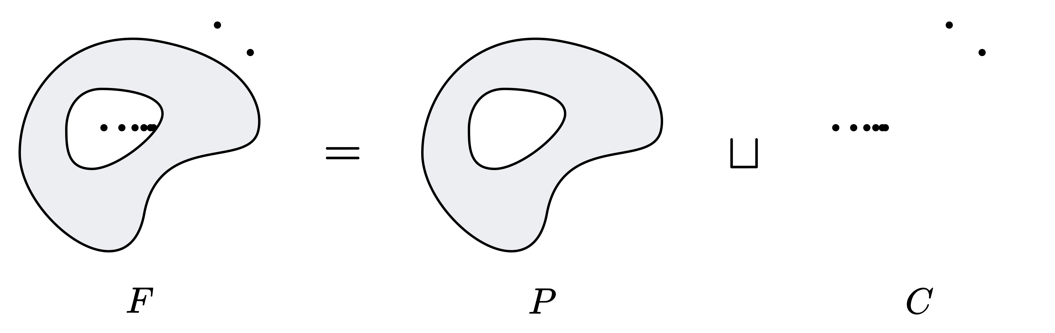
완벽한 집합은 고립점이 없는 닫힌 집합이므로, 위 정리는 “닫힌 집합은 최대 가산 개의 고립점을 가진다”로 재진술할 수 있다.

증명. 다음과 같이 $P, C$를 정의한다.

\[P = \lbrace x \in F : \text{For all nbd $U$ of $x$, $U \cap F$ is uncountable} \rbrace\] \[C = \lbrace x \in F : \text{There exists a nbd $U$ of $x$ s.t. $U \cap F$ is countable} \rbrace\]

$F = P \sqcup C$임에 주목하라.

Claim 1. $C$는 $F$에서 열린 집합이다.

Proof of Claim. $x \in C$일 때 어떤 $x$의 근방 $U$가 존재하여 $U \cap F$가 가산이다. 즉, 임의의 $y \in U \cap F$에 대해 $U$는 $y$의 근방이고 $U \cap F$가 가산이므로 $y \in C$이다. 따라서 $U \cap F \subset C$이다. □

Claim 2. $C$는 가산이다.

Proof of Claim. $F$의 부분공간 토폴로지를 생각하자. 가정에 의해 이 토폴로지는 린델뢰프이다. 임의의 $x \in C$에 대해 $U_x \cap F$가 가산인 $x$의 근방 $U_x$를 찾을 수 있다. 그러면 $\lbrace U_x \rbrace_{x \in C}$는 $C$의 $F$-열린 덮개이며, 린델뢰프 가정에 의해 $C = \bigcup_{\alpha \in J} U_\alpha$ ($J$는 가산)이다. $U_\alpha$가 가산이므로 $C$는 가산이다. □

Claim 3. $P$는 완벽하다.

Proof of Claim. Claim 1에 의해 $P$는 $F$에서 닫힌 집합이며, $F$가 닫힌 집합이므로 $P$는 $X$에서 닫힌 집합이다. 따라서 $P’ \subset P$이다. 역을 보이기 위해 $x \in P$라고 하자. 임의의 $x$의 근방 $U$에 대해 $U \cap F = (U \cap C) \sqcup (U \cap P)$가 비가산이다. $C$가 가산이므로, $U \cap P$가 비가산이어야 한다. 따라서 $U$는 $P$와 $\lbrace x \rbrace$보다 큰 교집합을 가지며, $x \in P’$이다. ■

정의. 분리 가능한_separable 완비 거리화 가능 공간을 폴란드 공간_{Polish space}이라고 한다.

거리화 가능 공간에서 분리 가능성, 2차 가산, 그리고 린델뢰프는 동치이므로 해당 세 가지 조건 중 하나로 정의를 대체할 수 있다. ‘폴란드 공간’이라는 이름은 해당 공간을 처음으로 연구한 학자들인 시에르핀스키, 쿠라토프스키, 타르스키 등이 폴란드인들인 데에서 유래했다.

$X$가 폴란드 공간이라는 더 강한 조건이 주어지면 칸토어-벤딕슨 분해가 유일함을 증명할 수 있다.

강한 칸토어-벤딕슨 정리. $X$가 폴란드 공간이라고 하자. $F \subset X$가 닫힌 집합일 때 어떤 완벽한 집합 $P$와 가산집합 $C$가 존재하여 $F = P \sqcup C$이다. 또한, 해당 분해는 유일하다.

또한 다음이 성립한다.

정리. 폴란드 공간의 완벽한 집합은 $2^{\aleph_0}$의 크기를 가진다.

증명. 추후 기술적 집합론에 대한 글에서 따로 다룰 예정.

이로부터 다음의 결론이 따라 나온다.

따름정리: 실수의 닫힌집합에서의 연속체 가설. 실수의 닫힌집합은 가산이거나 $2^{\aleph_0}$의 크기를 가진다.

증명. 실수는 폴란드 공간이므로 칸토어-벤딕슨 정리에 의해 모든 닫힌집합이 가산집합과 완벽한 집합의 서로소 합으로 분해된다. 후자가 공집합일 경우 해당 닫힌집합은 가산이며, 그렇지 않을 경우 $2^{\aleph_0}$이다. ■

칸토어는 위 정리의 증명으로부터 일반적인 연속체 가설을 증명할 수 있으리라는 희망을 품었지만 잘 알려져 있다시피 그 희망은 실현되지 못했다.

The Cantor-Bendixson Theorem and Polish Space

25 Dec 2024

This post was originally written in Korean, and has been machine translated into English. It may contain minor errors or unnatural expressions. Proofreading will be done in the near future.

Definition. A set $P$ in a topological space $X$ is perfect when $P’ = P$. Here, $P’$ denotes the set of limit points of $P$.

Remark. Every perfect set is a closed set, but the converse does not hold. Recall that in general $S \not\subset S’$ (when $S$ has isolated points) and $S’ \not\subset S$ (when $S$ is not a closed set). It follows that a perfect set is a closed set with no isolated points.

Definition. A topological space $X$ is hereditarily Lindelöf when every subspace of $X$ is Lindelöf.

Weak Cantor-Bendixson Theorem. Let $X$ be a hereditarily Lindelöf space. For any closed set $F \subset X$, there exist a perfect set $P$ and a countable set $C$ such that $F = P \sqcup C$.

Since a perfect space is a closed space with no isolated points, the above theorem can be restated as: A closed subspace of a hereditarily Lindelöf space has at most countable isolated points.

Proof. We define $P$ and $C$ as follows:

\[P = \lbrace x \in F : \text{For all nbd $U$ of $x$, $U \cap F$ is uncountable} \rbrace\] \[C = \lbrace x \in F : \text{There exists a nbd $U$ of $x$ s.t. $U \cap F$ is countable} \rbrace\]

Note that $F = P \sqcup C$.

Claim 1. $C$ is open in $F$.

Proof of Claim. When $x \in C$, there exists a neighbourhood $U$ of $x$ such that $U \cap F$ is countable. That is, for any $y \in U \cap F$, $U$ is a neighbourhood of $y$ and $U \cap F$ is countable, so $y \in C$. Therefore $U \cap F \subset C$. □

Claim 2. $C$ is countable.

Proof of Claim. Consider the subspace topology on $F$. By hypothesis, this topology is Lindelöf. For any $x \in C$, we can find a neighbourhood $U_x$ of $x$ such that $U_x \cap F$ is countable. Then $\lbrace U_x \rbrace_{x \in C}$ is an $F$-open cover of $C$, and by the Lindelöf hypothesis, $C = \bigcup_{\alpha \in J} U_\alpha$ where $J$ is countable. Since each $U_\alpha$ is countable, $C$ is countable. □

Claim 3. $P$ is perfect.

Proof of Claim. By Claim 1, $P$ is a closed set in $F$, and since $F$ is a closed set, $P$ is a closed set in $X$. Therefore $P’ \subset P$. To show the reverse inclusion, let $x \in P$. For any neighbourhood $U$ of $x$, we have that $U \cap F = (U \cap C) \sqcup (U \cap P)$ is uncountable. Since $C$ is countable, $U \cap P$ must be uncountable. Therefore $U$ has intersection with $P$ larger than $\lbrace x \rbrace$, and hence $x \in P’$. ■

Definition. A separable complete metrisable space is called a Polish space.

In metrisable spaces, separability, second countability, and the Lindelöf property are equivalent, so the definition can be replaced with any of these three conditions. The name ‘Polish space’ derives from the fact that the mathematicians who first studied these spaces — Sierpiński, Kuratowski, Tarski — were Polish.

When the stronger condition that $X$ is a Polish space is given, one can prove that the Cantor-Bendixson decomposition is unique.

Strong Cantor-Bendixson Theorem. Let $X$ be a Polish space. For any closed set $F \subset X$, there exist a perfect set $P$ and a countable set $C$ such that $F = P \sqcup C$. Moreover, this decomposition is unique.

The following also holds:

Theorem. A perfect set in a Polish space has cardinality $2^{\aleph_0}$.

Proof. This will be treated separately in a future article on descriptive set theory.

From this, the following conclusion follows:

Corollary: The Continuum Hypothesis for Closed Sets of Real Numbers. A closed set of real numbers is either countable or has cardinality $2^{\aleph_0}$.

Proof. Since the real numbers form a Polish space, by the Cantor-Bendixson theorem every closed set decomposes as a disjoint union of a countable set and a perfect set. If the latter is empty, then the closed set is countable; otherwise it has cardinality $2^{\aleph_0}$. ■

Cantor had hoped that from the proof of the above theorem he might be able to prove the general continuum hypothesis, but as is well known, this hope was not realised.

어드조인트에 대한 직관적 이해

16 Dec 2024

카테고리 이론의 핵심 개념 중 하나는 어드조인트_adjoint이다.

정의. $\mathcal{A}, \mathcal{B}$가 카테고리이고, $F: \mathcal{A} \to \mathcal{B}, G: \mathcal{B} \to \mathcal{A}$가 함자_functor라고 하자. $F$가 $G$의 좌 어드조인트_{left adjoint}라는 것은 임의의 $A \in \mathcal{A}, B \in \mathcal{B}$에 대해 $\mathcal{B}(F(A), B)$와 $\mathcal{A}(A, G(B))$가 자연스럽게 일대일 대응될 수 있다는 것이다. 즉,

\[\begin{gather} (F(A) \xrightarrow{g} B) \quad \mapsto \quad (A \xrightarrow{\bar{g}} G(B))\\ (A \xrightarrow{f} G(B)) \quad \mapsto \quad (F(A) \xrightarrow{\bar{f}} B) \end{gather}\]

또한 $G$를 $F$의 우 어드조인트_{right adjoint}라고 한다. 기호로 $F \dashv G$로 표기한다.

이 정의는 다소 추상적으로 느껴질 수 있지만, 이해를 돕는 몇 가지 직관이 있다.

1. 근사로서의 어드조인트

$F \dashv G$일 때 $F, G$는 $\mathcal{A}$과 $\mathcal{B}$의 원소들을 서로 근사하는 방법으로 생각할 수 있다. 특히 좌 어드조인트는 ‘좌측에서 우측으로‘의 근사이고, 우 어드조인트는 ‘우측에서 좌측으로’의 근사이다.

예를 들어 $\mathbf{Z}$가 정수를 원소로 가지고, $x \leq y$일 때 그리고 오직 그 경우에만 $x \to y$ 사상이 유일하게 존재하는 카테고리라고 하자. 또한 $\mathbf{R}$이 실수를 원소로 가지고, $x \leq y$일 때 그리고 오직 그 경우에만 $x \to y$ 사상이 유일하게 존재하는 카테고리라고 하자. 이때 $\lceil \cdot \rceil, \lfloor \cdot \rfloor$는 표준적인 방식으로 함자 $\mathbf{R} → \mathbf{Z}$가 되고, 포함 사상 $\iota$는 함자 $\mathbf{Z} → \mathbf{R}$이 된다. 또한 $\lceil \cdot \rceil \dashv \iota \dashv \lfloor \cdot \rfloor$임을 확인할 수 있다.

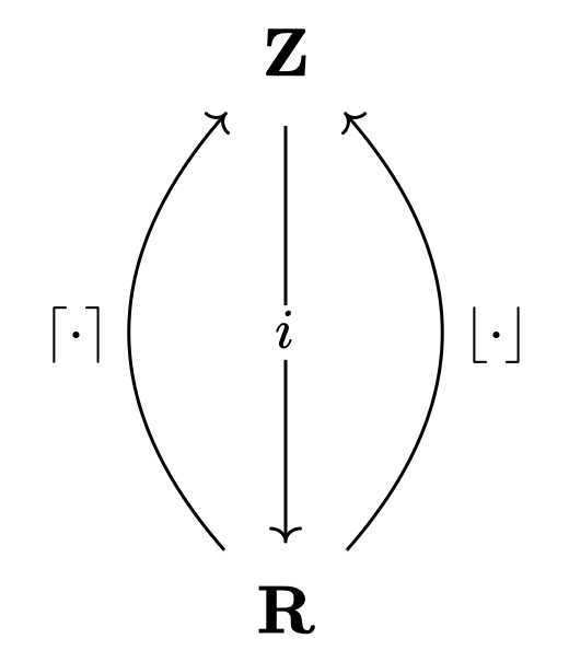
즉 $\lceil \cdot \rceil$는 $r$을 $r \leq \lceil r \rceil$로 ‘좌측에서 우측으로 끌어올리는’ 변환이고, $\lfloor \cdot \rfloor$은 $r$을 $\lfloor r \rfloor \leq r$로 ‘우측에서 좌측으로 잡아당기는’ 변환이다.

또한 $I, T$가 각각 $\mathcal{A}$의 초기 대상_{initial object} 및 종단 대상_{terminal object}라고 하자. 즉, 임의의 $A \in \mathcal{A}$에 대해

• 사상 $I \to A$가 유일하게 존재한다.
• 사상 $A \to T$가 유일하게 존재한다.

일례로 $\mathbf{Set}$에서 공집합은 초기 대상이고 홑원소 집합은 종단 대상이다.

홑원소 카테고리 $\mathcal{U}$에 대해 함자 $F: \mathcal{A} \to \mathcal{U}$가 유일하게 존재한다. $G_I, G_T: \mathcal{U} \to \mathcal{A}$가 각각 상이 $I, T$인 함자라고 하자. 이때 앞선 경우와 비슷한 원리로 $G_T \dashv F \dashv G_I$가 됨을 확인하라. (종단 대상은 가장 “오른쪽”에 있는 대상이므로 $G_T$는 “왼쪽에서 오른쪽으로”의 근사이며, 초기 대상은 가장 “왼쪽”에 있는 대상이므로 $G_I$는 “오른쪽에서 왼쪽으로”의 근사이다.)

2. 구축과 파괴로서의 어드조인트

좌 어드조인트는 구축을, 우 어드조인트는 파괴를 의미한다. 따라서 일반적으로 자유함자_{free functor}는 좌 어드조인트, 망각함자_{forgetful functor}는 우 어드조인트이다.

일례로 군의 카테고리를 $\mathbf{Grp}$, 모노이드의 카테고리를 $\mathbf{Mon}$이라 하자. $F$를 자유함자, $U$를 망각함자라고 하자. 그리고 $R: \mathbf{Mon} → \mathbf{Grp}$를 다음과 같이 정의한다.

• $R(M) = \lbrace m \in M : \exists m^{-1} \in M \rbrace$
• $R(f): m \mapsto f(m)$

이때, 다음 다이어그램이 성립하여 $F \dashv U \dashv R$이다.

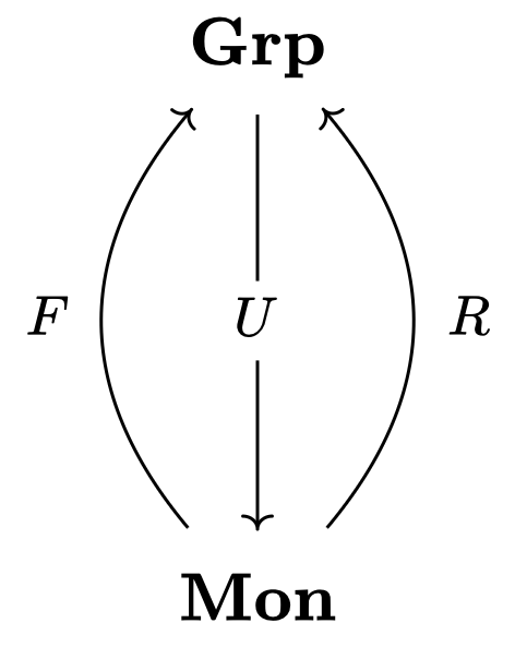
$R$이 $U$보다 더 파괴적이기 때문에 $U \dashv R$인 것으로 이해할 수 있다.

An Intuitive Understanding of Adjoints

16 Dec 2024

One of the central concepts in category theory is that of an adjoint.

Definition. Let $\mathcal{A}, \mathcal{B}$ be categories, and let $F: \mathcal{A} \to \mathcal{B}, G: \mathcal{B} \to \mathcal{A}$ be functors. We say that $F$ is a left adjoint to $G$, written as $F \dashv G$, if for any $A \in \mathcal{A}, B \in \mathcal{B}$, there exists a natural correspondence between $\hom_\mathcal{B}(F(A), B)$ and $\hom_\mathcal{A}(A, G(B))$. That is,

\[\begin{gather} (F(A) \xrightarrow{g} B) \quad \mapsto \quad (A \xrightarrow{\bar{g}} G(B))\\ (A \xrightarrow{f} G(B)) \quad \mapsto \quad (F(A) \xrightarrow{\bar{f}} B) \end{gather}\]

We also call $G$ the right adjoint to $F$.

This may feel very abstract, but there is a couple of examples that could be of assist in grasping the definition.

1. Adjoints as Approximations

When $F \dashv G$, the functors $F$ and $G$ can be thought of as approximating objects in $\mathcal{A}$ and $\mathcal{B}$ with respect to each other. In particular, the left adjoint represents approximation ‘from left to right’, while the right adjoint represents approximation ‘from right to left’.

For example, let $\mathbf{Z}$ be a category whose objects are integers, with a unique morphism $x \to y$ existing if and only if $x \leq y$. Similarly, let $\mathbf{R}$ be a category whose objects are real numbers, with a unique morphism $x \to y$ existing if and only if $x \leq y$. We may think of $\lceil \cdot \rceil, \lfloor \cdot \rfloor$ as functors $\mathbf{R} → \mathbf{Z}$, and the inclusion map $\iota$ as a functor $\mathbf{Z} → \mathbf{R}$. It then follows that $\lceil \cdot \rceil \dashv \iota \dashv \lfloor \cdot \rfloor$.

That is, $\lceil \cdot \rceil$ is a transformation that ‘lifts [a number] from left to right’ by mapping $r$ to $\lceil r \rceil$ with $r \leq \lceil r \rceil$, while $\lfloor \cdot \rfloor$ is a transformation that ‘pulls [a number] from right to left’ by mapping $r$ to $\lfloor r \rfloor$ with $\lfloor r \rfloor \leq r$.

Furthermore, let $I$ and $T$ be the initial object and terminal object of $\mathcal{A}$ respectively. That is, for any $A \in \mathcal{A}$:

• There exists a unique morphism $I \to A$.
• There exists a unique morphism $A \to T$.

For instance, in $\mathbf{Set}$, the empty set is the initial object and any singleton set is a terminal object.

For the singleton category $\mathcal{S}$, there exists a unique functor $F: \mathcal{A} \to \mathcal{S}$ that maps every object of $\mathcal{A}$ to the single object of $\mathcal{S}$. Let $G_I, G_T: \mathcal{S} \to \mathcal{A}$ be functors that maps the single object of $\mathcal{S}$ to $I$ and $T$, respectively. It then follows that $G_T \dashv F \dashv G_I$. (Since the terminal object is the ‘rightmost’ object, $G_T$ represents approximation ‘from left to right’, while since the initial object is the ‘leftmost’ object, $G_I$ represents approximation ‘from right to left’.)

2. Adjoints as Construction and Destruction

Left adjoints are associated with construction, while right adjoints are associated with destruction. Therefore, free functors are generally left adjoints, while forgetful functors are right adjoints.

For instance, let $\mathbf{Grp}$ be the category of groups and $\mathbf{Mon}$ be the category of monoids. Let $F$ be the free functor and $U$ be the forgetful functor. Define $R: \mathbf{Mon} → \mathbf{Grp}$ as follows:

• $R(M) = \lbrace m \in M : \exists m^{-1} \in M \rbrace$
• $R(f): m \mapsto f(m)$

Then the following diagram holds, yielding $F \dashv U \dashv R$.

One can understand $U \dashv R$ as expressing that $R$ is more destructive than $U$.

굴림에 대한 두 가지 삽화

11 Dec 2024

학부 시절 고전역학 수강 때 개인 공부용으로 만든 삽화인데, 잘 정리한 듯하여 이곳에도 공유한다.

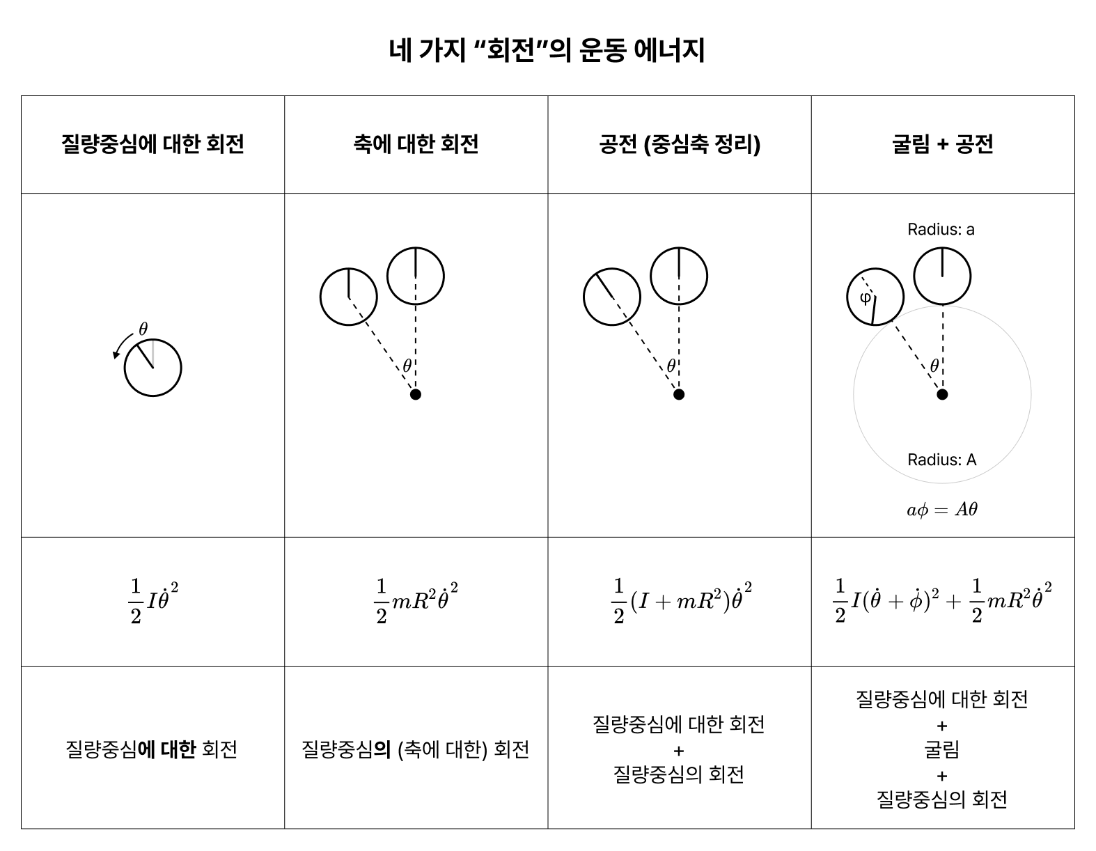
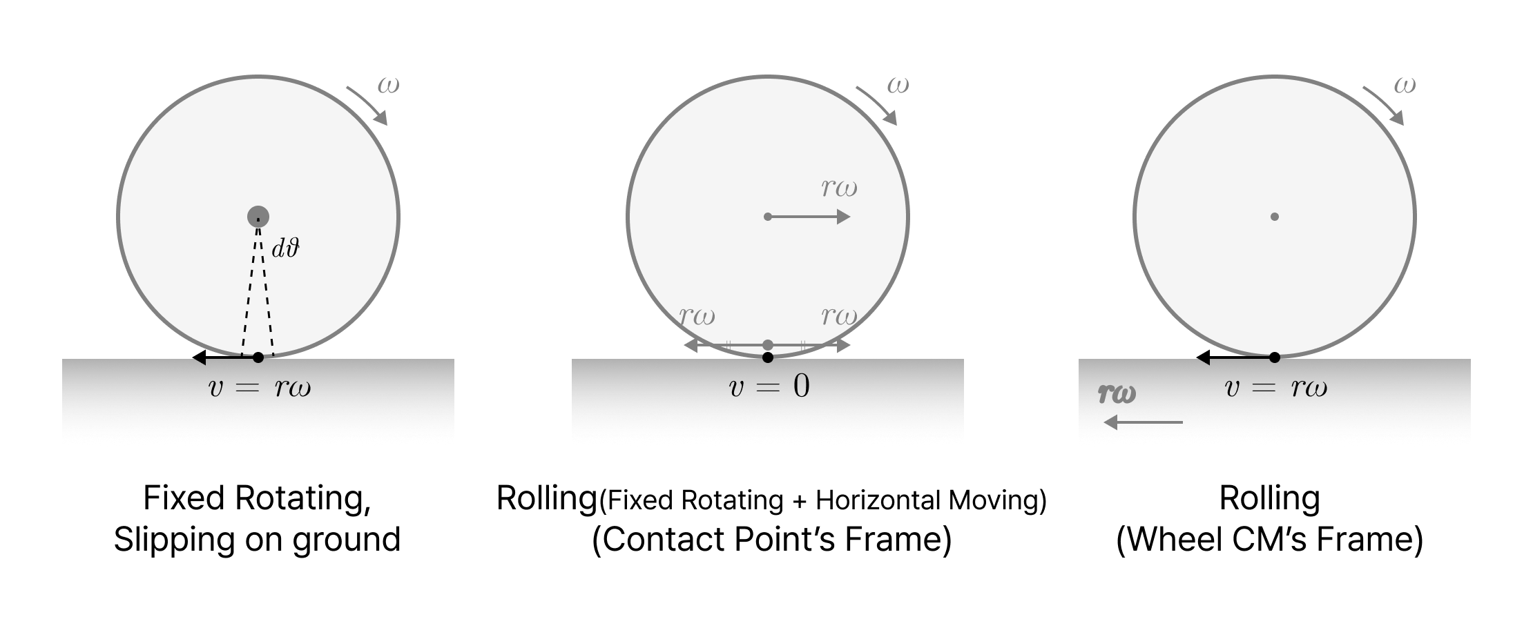
굴림을 바퀴의 CM 기준으로 분석할 때 땅 또한 움직인다는 사실에 유의하자.

Two Illustrations on Rolling

11 Dec 2024

These are illustrations I made when I studied classical mechanics in my BA. They seem to be well-made, so I decided to share them here, too.

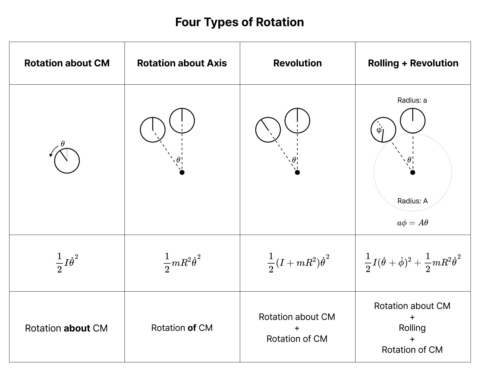
Note that decomposing Revolution as the sum of Rotation about CM and Rotation about Axis is a specific case of the central axis theorem.

Note that when analysing Rolling from CM’s frame, the ground also moves at $v = -r\omega$.

V = L 공리의 무모순성

11 Dec 2024

1. 전체

1.1. 폰 노이만 전체

초한귀납적으로 $\lbrace V_\alpha \rbrace$를 정의하자.

• $V_0 = \varnothing$
• $V_{\alpha + 1} = V_\alpha \cup \mathcal{P}(V_\alpha)$
• $\lambda$가 극한 서수일 때, $V_\lambda = \bigcup_{\alpha < \lambda} V_\alpha$

처음 몇 개의 $V_\alpha$는 다음과 같다.

• $V_1 = \lbrace \varnothing \rbrace$
• $V_2 = \lbrace \varnothing, \lbrace \varnothing \rbrace \rbrace$
• $V_3 = \lbrace \varnothing, \lbrace \varnothing \rbrace, \lbrace \lbrace \varnothing \rbrace \rbrace, \lbrace \varnothing, \lbrace \lbrace \varnothing\rbrace \rbrace \rbrace$
• $V_\omega = \mathsf{HF}$

모든 서수 $\alpha$에 대해 $V_\alpha$를 모아둔 모임을 폰 노이만 전체라고 한다.

\[V = \bigcup_{\alpha \in \mathrm{Ord}} V_\alpha\]

$x \in y \in z$가 $x \in z$를 시사할 때 $z$를 추이적 집합_{transitive set}이라고 한다. 이것은 $V$의 중요한 특징이다.

정리.

1. $\alpha \in \mathrm{Ord}$에 대해 $V_\alpha$는 추이적이다.
2. $V$는 추이적이다.

증명은 초한귀납법을 이용한다. 이에 따라 $V$를 다음과 같이 정의해도 무방하다.

• $V_0 = \varnothing$
• $V_{\alpha + 1} = \mathcal{P}(V_\alpha)$
• $\lambda$가 극한 서수일 때, $V_\lambda = \bigcup_{\alpha < \lambda}V_\alpha$

직관적으로 생각했을 때 $V$는 모든 집합을 포함하는 듯하다. 실제로 다음을 증명할 수 있다.

정리. $x$가 집합이라면 $x \in V$이다.

증명. 집합 $x$에 대해 $x$의 추이적 폐포 $\bar{x}$를, $x$를 원소로 가지는 가장 작은 추이적 집합으로 정의한다(이것이 well-defined임을 증명하기 위해서는 $x_0 = x, x_{n + 1} = \lbrace y : y \in x \text{ for some } x \in x_n \rbrace $일 때 $\bigcup x_n$가 $\bar{x}$임을 보이면 된다.)

$x \notin V$라고 가정하자. 분류 공리에 의해 $y = \lbrace u \in \bar{x} : u \notin V \rbrace$가 집합이며, 정초 공리에 의해 $y$의 $\in$-극소 원소 $z$가 존재한다. 만약 $w \notin V$인 $w \in z$가 존재한다면, 추이성에 의해 $w \in y$가 되어 $z$의 $\in$-극소성과 모순된다. 따라서 $z$의 모든 원소는 $V$에 있으며, 치환 공리로부터 $\Omega = \lbrace \alpha \in \mathrm{Ord} \mid \exists w \in z : w \in V_\alpha\rbrace$가 집합이다. $\beta = \bigcup_{\alpha \in \Omega}\alpha$라고 하자. $\beta$는 서수이며, $z \in V_{\beta + 1}$이다. (이 부분에서 $V_{\beta + 1} = \mathcal{P}(V_\beta)$임이 필요하다) 따라서 모순이다. ■

이에 따라 $V$는 집합이 아니다. 따라서 $V$는 모든 집합을 포함한다는 점에서 ZFC의 모델이지만, 많은 수학자들은 모델이 집합일 것을 요구하기 때문에 엄격한 의미에서의 모델은 아니다. 나중에 드러나겠지만, 이는 $V = L$의 무모순성 증명이 괴델의 제2불완전성 정리와 상충하지 않는 이유를 설명한다.

한편 $x \in V$는 “$x$는 집합이다“의 형식적 표현으로 이해하도록 한다.

1.2. 괴델 구성 가능 전체

먼저 다음과 같이 구성 가능성을 정의한다.

정의. 집합론의 언어를 $\mathcal{L}$이라고 하자. $X$가 $\mathcal{L}$-구조 $(L, \in)$에서 구성 가능하다는 것은, 어떤 $\mathcal{L}$-명제 $\phi$와 자유변수 할당 $g$가 존재하여 다음이 성립한다는 것이다.

\[X = \{ x \in L : (L, \in) \vDash \phi[g^0_x] \}\]

예를 들어 $L = \lbrace 0, 1, 2\rbrace$일 때 다음은 $X = \lbrace 1, 2 \rbrace$를 구성한다.

• $\phi(v_0, v_1, v_2) := (v_0 = v_1) \lor (v_0 = v_2)$
• $g: v_1 \mapsto 1, v_2 \mapsto 2$

또한 $L = \mathbb{N}$일 때 다음은 $X = \lbrace 0, 3, 6, 9, \dots \rbrace$를 구성한다.

• $\phi(v_0, v_1) := v_1 \mid v_0$
• $g: v_1 \mapsto 3$

괴델의 구성가능성은 언어로서의 표현가능성과 다르다. 일례로 언어로 표현가능한 실수의 집합은 가산이므로, 어떤 실수는 언어로 표현이 불가능하다. 그러한 실수를 $r$이라고 하자. $(L, \in)$이 실수 집합을 포함하는 구조일 때, 다음은 $X = \lbrace r \rbrace$을 구성한다.

• $\phi(v_0, v_1) := v_0 = v_1$
• $g: v_1 \mapsto r$

즉, 괴델의 구성가능성은 자유변수의 초기화를 임의의 원소에 대해 허용한다는 점에서 강력하다. 그러나 자유변수의 수가 유한하다는 점에서 한계를 가진다. 이제 초한귀납적으로 $\lbrace L_\alpha \rbrace$를 정의하자.

• $L_0 = \varnothing$
• $L_{\alpha + 1} = \lbrace x : x \text{ is constructible from } (L_\alpha, \in) \rbrace$
• $\lambda$가 극한 서수일 때, $L_\lambda = \bigcup_{\alpha < \lambda} L_\alpha$
• $L = \bigcup_{\alpha \in \mathrm{Ord}} L_\alpha$

$\alpha < \omega$일 때 $L_\alpha = V_\alpha$임을 쉽게 보일 수 있다. $\alpha = n$일 때, 최대 $n$개의 $\lor$ 연언으로 $x \in V_\alpha$를 구성할 수 있기 때문이다. 따라서,

• $L_1 = \lbrace \varnothing \rbrace$
• $L_2 = \lbrace \varnothing, \lbrace \varnothing \rbrace \rbrace$
• $L_3 = \lbrace \varnothing, \lbrace \varnothing \rbrace, \lbrace \lbrace \varnothing \rbrace \rbrace, \lbrace \varnothing, \lbrace \lbrace \varnothing\rbrace \rbrace \rbrace$
• $L_\omega = \mathsf{HF}$

하지만 $L_{\omega + 1} \subsetneq V_{\omega + 1}$이다. $\mathcal{P}(\mathbb{N}) \subset V_{\omega + 1}$이므로 $V_{\omega + 1}$은 비가산인 반면, 1차 논리 문장들의 집합과 $L_\omega$는 모두 가산이므로 $L_{\omega + 1}$ 또한 가산이기 때문이다. 일반적으로 $\alpha$가 가산일 때 $L_\alpha$는 가산이다.

그럼에도 $L$은 $V$와 많은 특징을 공유한다. 일례로,

정리. $\alpha \in \mathrm{Ord}$에 대해 다음이 성립한다.

1. $L_\alpha$는 추이적이다. (따라서 $L$이 추이적이다)
2. $\alpha \in L_{\alpha + 1} \setminus L_{\alpha}$

증명은 초한귀납법을 사용한다.

$L$은 모든 서수를 포함하므로 부랄리포르티 정리에 의해 집합이 아님에 유의하라. 대신 $x \in L_\alpha$에 대응되는 1차 논리식 $\mathsf{IsInL}_\alpha(x)$가 존재한다. 증명은 조금 까다로운데, 괴델 수를 이용하여 명제를 산술화하면 된다. (링크 참조) 따라서 $x \in L$을 $\exists \alpha \in \mathrm{Ord} :\mathsf{IsInL}_\alpha(x)$를 대체하는 형식적 표현으로 이해하여 사용하도록 한다. (물론 $\alpha \in \mathrm{Ord}$ 또한 1차 논리식을 대체하는 형식적 표현으로 이해되어야 한다)

2. 상대화

2.1. 명제의 상대화

1차 논리 명제는 양화사를 포함할 수 있다. 때문에 양화사의 정의역을 어떻게 설정하느냐의 따라 명제의 의미가 달라진다.

명제 $\phi$와 집합 (또는 모임) $A$에 대해, $\phi$의 상대화 $\phi^A$를 $\phi$의 모든 양화사를 $A$로 제한한 명제로 정의한다. 약간의 서사적 표현을 곁들이자면, $\phi^A$는 $A$의 “내부”에서 이해한 $\phi$라고 할 수 있겠다. 예를 들어, $\phi : \forall x \; \exists y : y < x$일 때

• $\phi^\mathbb{N} : \forall x \in \mathbb{N} \; \exists y \in \mathbb{N} : y < x$
• $\phi^\mathbb{Z} : \forall x \in \mathbb{Z} \; \exists y \in \mathbb{Z} : y < x$

$T_\mathbb{Q}$가 자연수 및 정수를 특정할 수 있는 정도의 표현력을 지니는 유리수 이론이라고 하면,

• $T_\mathbb{Q} \vdash \phi$
• $T_\mathbb{Q} \not\vdash \phi^\mathbb{N}$
• $T_\mathbb{Q} \vdash \phi^{\mathbb{Z}}$

이다. 따라서 $\phi$는 자연수와 유리수를 성공적으로 구분해 내지만, 정수와 유리수는 구분해 내지 못한다. 이 관찰을 일반화하면, 이론 $T$와 집합 $A$에 대해 $T \vdash \phi \leftrightarrow \phi^A$인 $\phi$가 많으면 많을수록 $A$는 $T$의 기술에 잘 “부합한다“고 말할 수 있다.

위 논의를 조금 일반화하여, 다음과 같이 정의한다.

정의. 이론 $T$와 집합 $A$에 대해서

\[T \vdash \forall x_1, \dots, x_n \in A (\phi(x_1, \dots, x_n) \leftrightarrow \phi^A(x_1, \dots, x_n))\]

일 때, $\phi$는 $A$에 대해 절대적_absolute이라고 한다.

일례로 $T_\mathbb{Q}$에 대해 $\phi(x) : \exists y (y < x)$는 정수에 대해 절대적이지만 자연수에 대해 절대적이지는 않다.

2.2. $L$-상대화

이제 우리의 목표는 $L$이 $\mathsf{ZF}$와 극대적으로 부합함을 보이는 것이다. 즉,

정리 1. $\phi$가 ZF의 공리라면 $\mathsf{ZF} \vdash \phi^L$이다.

정리 1의 의미를 말로 풀어 보자면,

“$L$의 내부에서 보았을 때 $L$은 ZF의 모델이다”를 ZF로 증명할 수 있다.

물론 우리는 $L \subset V$만 알고 $V = L$인지는 알지 못하기 때문에, 어떤 집합 $x$는 $L$에 속하지 않을 수도 있다. 그러나 설령 $x \in V \setminus L$인 집합 $x$가 있더라도, 그러한 $x$의 결여는 $L$의 내적 정합성을 깨뜨리지 않는다는 것이 정리 1의 내용이다.

예를 들어 어떤 집합 $y, z$에 대해 $x = \lbrace y, z \rbrace$가 $L$에 결여되어 있다고 하자. 일면 $x$의 결여는 $L$이 짝 공리 $\mathsf{Pair}$을 만족하지 않음을 시사하는 듯하다.

\[\mathsf{Pair} := \forall y, z \; \exists x \; \forall w: w \in x \leftrightarrow (w = y \lor w = z)\]

하지만 $L$의 내부에서 본 짝 공리는 다음과 같다.

\[\mathsf{Pair}^L := \forall y, z \in L \; \exists x \in L \; \forall w \in L: w \in x \leftrightarrow (w = y \lor w = z)\]

$\forall y, z$의 양화 또한 $L$로 한정됨에 주목하라. 즉, $x = \lbrace y, z \rbrace$의 결여가 $L$에게 문제를 일으키는 경우는 $y, z \in L$일 때이다. 거꾸로 말해, $x = \lbrace y, z \rbrace \notin L$이 $y, z \notin L$을 시사한다면 $L$은 $\mathsf{Pair}^L$을 만족한다. 이것이 “$L$이 내적 정합성을 유지하는 방식으로 집합을 결여한다”의 의미이다.

정리 1이 성립하는 핵심 이유는 $L$과 $V$가 추이성이라는 성질을 공유하기 때문이다.

보조정리. 다음 술어는 ZF에서 $L$에 대해 절대적이다.

1. $x \in y$
2. $x \subset y$
3. $x = \bigcup y$
4. $x = \lbrace y, z \rbrace$
5. $\alpha \in \mathrm{Ord}$
6. $x$는 추이적이다.
7. $\Delta_0$ 논리식

또한 다음을 증명할 수 있다.

정리 2. $\mathsf{ZF} \vdash (V = L)^L$

여기서 $V = L$은, “모든 집합이 $L$에 속한다”를 의미한다. 따라서 일면 보기에 $(V = L)^L$은 “$L$에 속하는 모든 집합이 $L$에 속한다”라는 자명한 명제인 듯하다. 하지만 실제로 $V = L$을 논리식으로 적으면

\[\forall x \; \exists \alpha : \alpha \in \mathrm{Ord} \land x \in L_\alpha\]

이므로 $(V = L)^L$은

\[\forall x \in L \; \exists \alpha \in L : (\alpha \in \mathrm{Ord})^L \land (x \in L_\alpha)^L\]

이다. 특히, $\alpha \in \mathrm{Ord}$와 $x \in L_\alpha$가 진정한 의미에서의 $\in$-술어가 아닌 1차 논리식의 형식적 표현이기 때문에 마찬가지로 $L$로 상대화해야 함에 유의하라. 이에 따라 $(V = L)^L$을 ZF에서 증명하기 위해서는 $\alpha \in \mathsf{Ord}$와 $x \in L_\alpha$가 절대적임을 증명해야 한다. 두 증명 모두 초한귀납법을 사용하면 가능하다.

정리 1과 정리 2로부터 다음을 증명할 수 있다.

정리 3. $\mathsf{ZFL} \vdash \phi \implies \mathsf{ZF} \vdash \phi^L$

증명. $\mathsf{ZFL} \vdash \phi$의 증명 길이에 대한 귀납법으로 증명한다. 증명 길이가 0일 때 $\phi$는 ZFL의 공리이다. $\phi$가 ZF의 공리일 때 정리 1로부터 증명되고, $\phi$가 $V = L$일 때 정리 2로부터 증명된다.

이제 $\phi$가 $\lbrace \psi_1, \dots, \psi_n \rbrace$에 추론 규칙을 적용하는 것으로 증명된다고 가정하자. $\psi_k$의 증명 길이는 $\phi$보다 작으므로 귀납 가정에 의해 $\mathsf{ZF} \vdash \psi_k^L$이며, 논리 공리와 추론 규칙은 $L$에 대해 절대적임을 쉽게 보일 수 있다. 따라서 $(\psi_1 \land \dots \land \psi_n) \rightarrow \phi$가 논리적 참이라면 $(\psi_1^L \land \dots \land \psi_n^L) → \phi^L$ 또한 논리적 참이며, 이에 따라 $\mathsf{ZF} \vdash \phi^L$이다. ■

정리 3의 따름정리로서 정리 4를 얻는다.

정리 4. ZF가 무모순적이라면 ZFL 또한 무모순적이다.

증명. ZFL이 모순적이라면 $\mathsf{ZFL} \vdash \varnothing \neq \varnothing$이며, 정리 3에 의해 $\mathsf{ZF} \vdash (\varnothing \neq \varnothing)^L \iff \mathsf{ZF} \vdash \varnothing \neq \varnothing$이다.

따라서 V = L은 ZF와 일관적이다.