Proving the Uncountability of Real Numbers Without the Diagonal Argument

26 Dec 2024

Theorem. $\mathbb{R}$ is uncountable. That is, there exists no surjective function from $\mathbb{N}$ to $\mathbb{R}$.

This is a theorem that any sophomore student would have encountered at least once. The most widely known proof is Cantor’s diagonal argument. However, there are methods to prove this theorem without the diagonal argument. These utilise the order-theoretic and topological properties of $\mathbb{R}$, respectively.

1. Proof Using the Isomorphism Theorem

Cantor’s isomorphism theorem states that all totally ordered sets $(S, \leq)$ satisfying the following conditions are order isomorphic:

1. $S$ is countable.
2. $S$ is dense. That is, for $x, y \in S$ with $x < y$, there exists $z \in S$ such that $x < z < y$.
3. $S$ has neither an upper bound nor a lower bound.

$(\mathbb{Q}, \leq)$ satisfies all three conditions above, while $(\mathbb{R}, \leq)$ satisfies conditions 2 and 3. Therefore, if $\mathbb{R}$ were countable, then $(\mathbb{R}, \leq)$ would be order isomorphic to $(\mathbb{Q}, \leq)$. However, the former is complete while the latter is not, so $\mathbb{R}$ is uncountable. ■

2. Proof Using Compactness

Let $X$ be a compact Hausdorff space with no isolated points. Also assume that $X \neq \varnothing$.

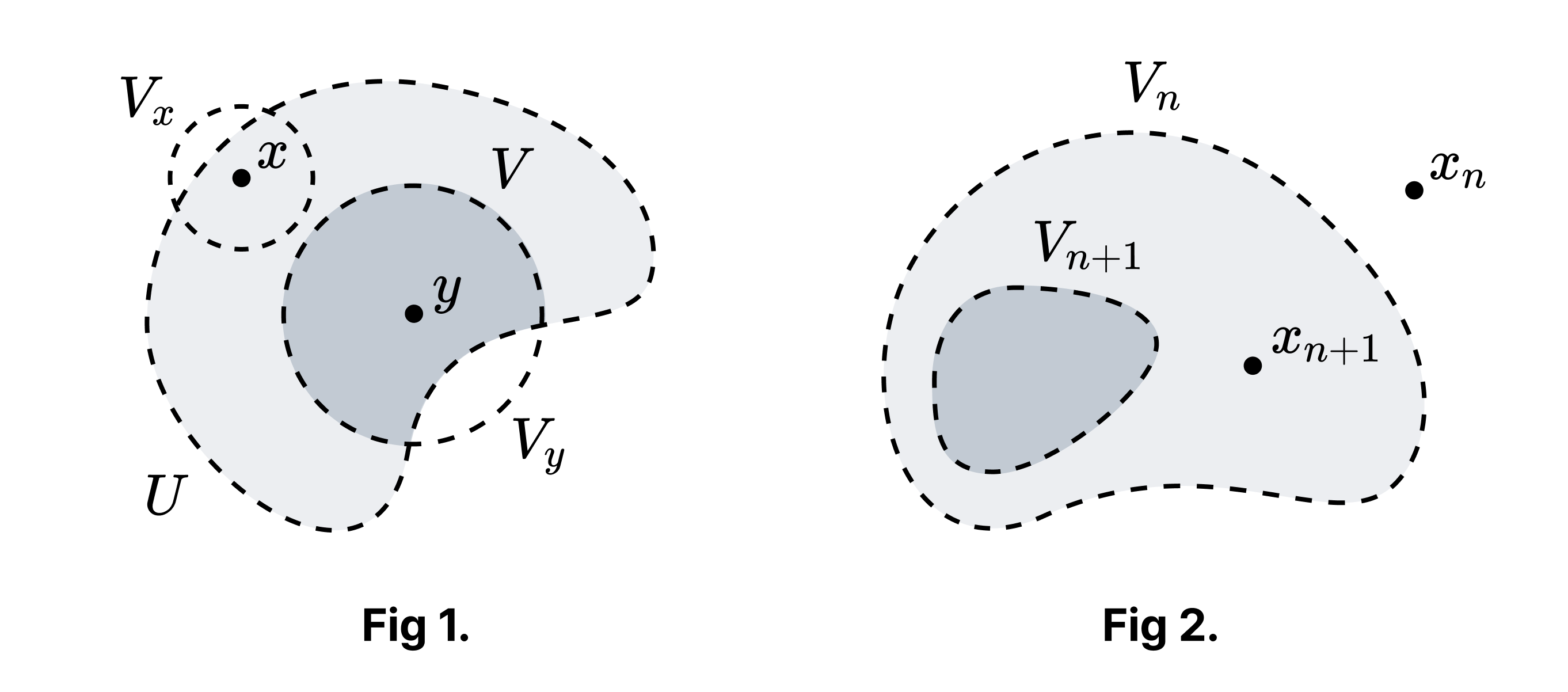
Claim 1. Let $U \neq \varnothing$ be an open subset of $X$. For $x \in X$, there exists an open set $V$ such that $x \notin \bar{V}$ and $V \subset U$.

Proof of Claim 1. There exists $y \in U$ where $x \neq y$. This is because if $x \in U$, then since $X$ has no isolated points such a $y$ must exist, and if $x \notin U$, then such a $y$ exists because $U$ is non-empty. Since $X$ is Hausdorff, we can separate $x$ and $y$ by neighbourhoods $V_x$ and $V_y$. Then $V = V_y \cap U$ is the desired set (the dark shaded region in Fig 1). □

Claim 2. $X$ is uncountable.

Proof of Claim 2. Suppose $X$ is countable. Enumerate the elements of $X$ as $\lbrace x_n\rbrace _{n \in \mathbb{Z}^+}$. Let $V_0 = X$. By Claim 1, for each $n$ there exists an open set $V_n$ such that $x_n \notin \bar{V_n}$ and $V_n \subset V_{n-1}$ (Fig 2). Since $X$ is compact, by the finite intersection property we have

\[K = \bigcap_{n \in \mathbb{Z}^+} \bar{V}_n \neq \varnothing.\]

However, if $x_n \in K$, then $x_n \in \bar{V}_n$, which is a contradiction. Therefore, $X$ is uncountable. □

Claim 3. $\mathbb{R}$ is uncountable.

Proof of Claim 3. $[0, 1]$ is a compact Hausdorff space with no isolated points. Therefore, it is uncountable. Consequently, $\mathbb{R}$ is uncountable. ■

칸토어-벤딕슨 정리와 폴란드 공간

25 Dec 2024

정의. 위상공간 $X$의 집합 $P$에 대해 $P’ = P$일 때 $P$를 완벽한 집합_{perfect set}이라고 한다. ($P’$은 $P$의 집적점들의 집합)

Remark. 모든 완벽한 집합은 닫힌 집합이지만, 역은 성립하지 않는다. 일반적으로 $S \not\subset S’$ ($S$가 고립점을 가짐), $S’ \not\subset S$ ($S$가 닫힌 집합이 아님) 임에 유의하라. 뒤집어 말해, 완벽한 집합은 고립점이 없는 닫힌 집합이다.

정의. $X$의 임의의 부분공간이 린델뢰프일 때 $X$를 세습적 린델뢰프_{hereditarily Lindelöf}라고 한다.

약한 칸토어-벤딕슨 정리. $X$가 세습적 린델뢰프 공간이라고 하자. $F \subset X$가 닫힌 집합일 때 어떤 완벽한 집합 $P$와 가산집합 $C$가 존재하여 $F = P \sqcup C$이다.

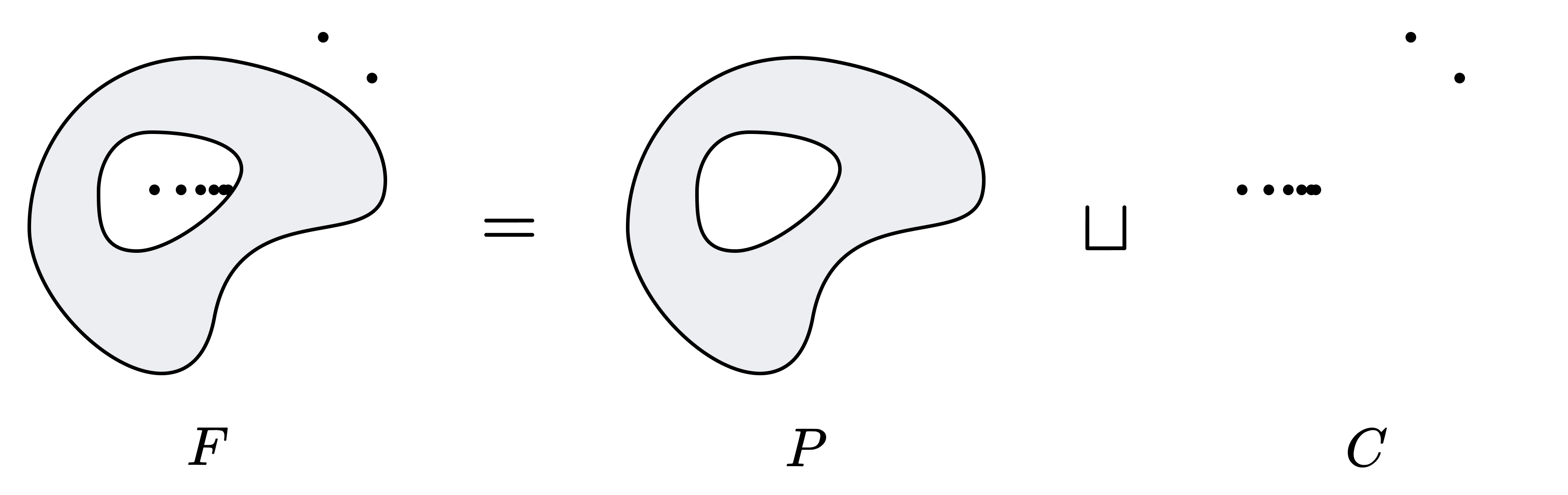
완벽한 집합은 고립점이 없는 닫힌 집합이므로, 위 정리는 “닫힌 집합은 최대 가산 개의 고립점을 가진다”로 재진술할 수 있다.

증명. 다음과 같이 $P, C$를 정의한다.

\[P = \lbrace x \in F : \text{For all nbd $U$ of $x$, $U \cap F$ is uncountable} \rbrace\] \[C = \lbrace x \in F : \text{There exists a nbd $U$ of $x$ s.t. $U \cap F$ is countable} \rbrace\]

$F = P \sqcup C$임에 주목하라.

Claim 1. $C$는 $F$에서 열린 집합이다.

Proof of Claim. $x \in C$일 때 어떤 $x$의 근방 $U$가 존재하여 $U \cap F$가 가산이다. 즉, 임의의 $y \in U \cap F$에 대해 $U$는 $y$의 근방이고 $U \cap F$가 가산이므로 $y \in C$이다. 따라서 $U \cap F \subset C$이다. □

Claim 2. $C$는 가산이다.

Proof of Claim. $F$의 부분공간 토폴로지를 생각하자. 가정에 의해 이 토폴로지는 린델뢰프이다. 임의의 $x \in C$에 대해 $U_x \cap F$가 가산인 $x$의 근방 $U_x$를 찾을 수 있다. 그러면 $\lbrace U_x \rbrace_{x \in C}$는 $C$의 $F$-열린 덮개이며, 린델뢰프 가정에 의해 $C = \bigcup_{\alpha \in J} U_\alpha$ ($J$는 가산)이다. $U_\alpha$가 가산이므로 $C$는 가산이다. □

Claim 3. $P$는 완벽하다.

Proof of Claim. Claim 1에 의해 $P$는 $F$에서 닫힌 집합이며, $F$가 닫힌 집합이므로 $P$는 $X$에서 닫힌 집합이다. 따라서 $P’ \subset P$이다. 역을 보이기 위해 $x \in P$라고 하자. 임의의 $x$의 근방 $U$에 대해 $U \cap F = (U \cap C) \sqcup (U \cap P)$가 비가산이다. $C$가 가산이므로, $U \cap P$가 비가산이어야 한다. 따라서 $U$는 $P$와 $\lbrace x \rbrace$보다 큰 교집합을 가지며, $x \in P’$이다. ■

정의. 분리 가능한_separable 완비 거리화 가능 공간을 폴란드 공간_{Polish space}이라고 한다.

거리화 가능 공간에서 분리 가능성, 2차 가산, 그리고 린델뢰프는 동치이므로 해당 세 가지 조건 중 하나로 정의를 대체할 수 있다. ‘폴란드 공간’이라는 이름은 해당 공간을 처음으로 연구한 학자들인 시에르핀스키, 쿠라토프스키, 타르스키 등이 폴란드인들인 데에서 유래했다.

$X$가 폴란드 공간이라는 더 강한 조건이 주어지면 칸토어-벤딕슨 분해가 유일함을 증명할 수 있다.

강한 칸토어-벤딕슨 정리. $X$가 폴란드 공간이라고 하자. $F \subset X$가 닫힌 집합일 때 어떤 완벽한 집합 $P$와 가산집합 $C$가 존재하여 $F = P \sqcup C$이다. 또한, 해당 분해는 유일하다.

또한 다음이 성립한다.

정리. 폴란드 공간의 완벽한 집합은 $2^{\aleph_0}$의 크기를 가진다.

증명. 추후 기술적 집합론에 대한 글에서 따로 다룰 예정.

이로부터 다음의 결론이 따라 나온다.

따름정리: 실수의 닫힌집합에서의 연속체 가설. 실수의 닫힌집합은 가산이거나 $2^{\aleph_0}$의 크기를 가진다.

증명. 실수는 폴란드 공간이므로 칸토어-벤딕슨 정리에 의해 모든 닫힌집합이 가산집합과 완벽한 집합의 서로소 합으로 분해된다. 후자가 공집합일 경우 해당 닫힌집합은 가산이며, 그렇지 않을 경우 $2^{\aleph_0}$이다. ■

칸토어는 위 정리의 증명으로부터 일반적인 연속체 가설을 증명할 수 있으리라는 희망을 품었지만 잘 알려져 있다시피 그 희망은 실현되지 못했다.

The Cantor-Bendixson Theorem and Polish Space

25 Dec 2024

This post was originally written in Korean, and has been machine translated into English. It may contain minor errors or unnatural expressions. Proofreading will be done in the near future.

Definition. A set $P$ in a topological space $X$ is perfect when $P’ = P$. Here, $P’$ denotes the set of limit points of $P$.

Remark. Every perfect set is a closed set, but the converse does not hold. Recall that in general $S \not\subset S’$ (when $S$ has isolated points) and $S’ \not\subset S$ (when $S$ is not a closed set). It follows that a perfect set is a closed set with no isolated points.

Definition. A topological space $X$ is hereditarily Lindelöf when every subspace of $X$ is Lindelöf.

Weak Cantor-Bendixson Theorem. Let $X$ be a hereditarily Lindelöf space. For any closed set $F \subset X$, there exist a perfect set $P$ and a countable set $C$ such that $F = P \sqcup C$.

Since a perfect space is a closed space with no isolated points, the above theorem can be restated as: A closed subspace of a hereditarily Lindelöf space has at most countable isolated points.

Proof. We define $P$ and $C$ as follows:

\[P = \lbrace x \in F : \text{For all nbd $U$ of $x$, $U \cap F$ is uncountable} \rbrace\] \[C = \lbrace x \in F : \text{There exists a nbd $U$ of $x$ s.t. $U \cap F$ is countable} \rbrace\]

Note that $F = P \sqcup C$.

Claim 1. $C$ is open in $F$.

Proof of Claim. When $x \in C$, there exists a neighbourhood $U$ of $x$ such that $U \cap F$ is countable. That is, for any $y \in U \cap F$, $U$ is a neighbourhood of $y$ and $U \cap F$ is countable, so $y \in C$. Therefore $U \cap F \subset C$. □

Claim 2. $C$ is countable.

Proof of Claim. Consider the subspace topology on $F$. By hypothesis, this topology is Lindelöf. For any $x \in C$, we can find a neighbourhood $U_x$ of $x$ such that $U_x \cap F$ is countable. Then $\lbrace U_x \rbrace_{x \in C}$ is an $F$-open cover of $C$, and by the Lindelöf hypothesis, $C = \bigcup_{\alpha \in J} U_\alpha$ where $J$ is countable. Since each $U_\alpha$ is countable, $C$ is countable. □

Claim 3. $P$ is perfect.

Proof of Claim. By Claim 1, $P$ is a closed set in $F$, and since $F$ is a closed set, $P$ is a closed set in $X$. Therefore $P’ \subset P$. To show the reverse inclusion, let $x \in P$. For any neighbourhood $U$ of $x$, we have that $U \cap F = (U \cap C) \sqcup (U \cap P)$ is uncountable. Since $C$ is countable, $U \cap P$ must be uncountable. Therefore $U$ has intersection with $P$ larger than $\lbrace x \rbrace$, and hence $x \in P’$. ■

Definition. A separable complete metrisable space is called a Polish space.

In metrisable spaces, separability, second countability, and the Lindelöf property are equivalent, so the definition can be replaced with any of these three conditions. The name ‘Polish space’ derives from the fact that the mathematicians who first studied these spaces — Sierpiński, Kuratowski, Tarski — were Polish.

When the stronger condition that $X$ is a Polish space is given, one can prove that the Cantor-Bendixson decomposition is unique.

Strong Cantor-Bendixson Theorem. Let $X$ be a Polish space. For any closed set $F \subset X$, there exist a perfect set $P$ and a countable set $C$ such that $F = P \sqcup C$. Moreover, this decomposition is unique.

The following also holds:

Theorem. A perfect set in a Polish space has cardinality $2^{\aleph_0}$.

Proof. This will be treated separately in a future article on descriptive set theory.

From this, the following conclusion follows:

Corollary: The Continuum Hypothesis for Closed Sets of Real Numbers. A closed set of real numbers is either countable or has cardinality $2^{\aleph_0}$.

Proof. Since the real numbers form a Polish space, by the Cantor-Bendixson theorem every closed set decomposes as a disjoint union of a countable set and a perfect set. If the latter is empty, then the closed set is countable; otherwise it has cardinality $2^{\aleph_0}$. ■

Cantor had hoped that from the proof of the above theorem he might be able to prove the general continuum hypothesis, but as is well known, this hope was not realised.

어드조인트에 대한 직관적 이해

16 Dec 2024

카테고리 이론의 핵심 개념 중 하나는 어드조인트_adjoint이다.

정의. $\mathcal{A}, \mathcal{B}$가 카테고리이고, $F: \mathcal{A} \to \mathcal{B}, G: \mathcal{B} \to \mathcal{A}$가 함자_functor라고 하자. $F$가 $G$의 좌 어드조인트_{left adjoint}라는 것은 임의의 $A \in \mathcal{A}, B \in \mathcal{B}$에 대해 $\mathcal{B}(F(A), B)$와 $\mathcal{A}(A, G(B))$가 자연스럽게 일대일 대응될 수 있다는 것이다. 즉,

\[\begin{gather} (F(A) \xrightarrow{g} B) \quad \mapsto \quad (A \xrightarrow{\bar{g}} G(B))\\ (A \xrightarrow{f} G(B)) \quad \mapsto \quad (F(A) \xrightarrow{\bar{f}} B) \end{gather}\]

또한 $G$를 $F$의 우 어드조인트_{right adjoint}라고 한다. 기호로 $F \dashv G$로 표기한다.

이 정의는 다소 추상적으로 느껴질 수 있지만, 이해를 돕는 몇 가지 직관이 있다.

1. 근사로서의 어드조인트

$F \dashv G$일 때 $F, G$는 $\mathcal{A}$과 $\mathcal{B}$의 원소들을 서로 근사하는 방법으로 생각할 수 있다. 특히 좌 어드조인트는 ‘좌측에서 우측으로‘의 근사이고, 우 어드조인트는 ‘우측에서 좌측으로’의 근사이다.

예를 들어 $\mathbf{Z}$가 정수를 원소로 가지고, $x \leq y$일 때 그리고 오직 그 경우에만 $x \to y$ 사상이 유일하게 존재하는 카테고리라고 하자. 또한 $\mathbf{R}$이 실수를 원소로 가지고, $x \leq y$일 때 그리고 오직 그 경우에만 $x \to y$ 사상이 유일하게 존재하는 카테고리라고 하자. 이때 $\lceil \cdot \rceil, \lfloor \cdot \rfloor$는 표준적인 방식으로 함자 $\mathbf{R} → \mathbf{Z}$가 되고, 포함 사상 $\iota$는 함자 $\mathbf{Z} → \mathbf{R}$이 된다. 또한 $\lceil \cdot \rceil \dashv \iota \dashv \lfloor \cdot \rfloor$임을 확인할 수 있다.

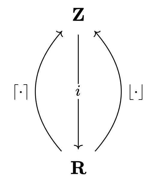
즉 $\lceil \cdot \rceil$는 $r$을 $r \leq \lceil r \rceil$로 ‘좌측에서 우측으로 끌어올리는’ 변환이고, $\lfloor \cdot \rfloor$은 $r$을 $\lfloor r \rfloor \leq r$로 ‘우측에서 좌측으로 잡아당기는’ 변환이다.

또한 $I, T$가 각각 $\mathcal{A}$의 초기 대상_{initial object} 및 종단 대상_{terminal object}라고 하자. 즉, 임의의 $A \in \mathcal{A}$에 대해

• 사상 $I \to A$가 유일하게 존재한다.
• 사상 $A \to T$가 유일하게 존재한다.

일례로 $\mathbf{Set}$에서 공집합은 초기 대상이고 홑원소 집합은 종단 대상이다.

홑원소 카테고리 $\mathcal{U}$에 대해 함자 $F: \mathcal{A} \to \mathcal{U}$가 유일하게 존재한다. $G_I, G_T: \mathcal{U} \to \mathcal{A}$가 각각 상이 $I, T$인 함자라고 하자. 이때 앞선 경우와 비슷한 원리로 $G_T \dashv F \dashv G_I$가 됨을 확인하라. (종단 대상은 가장 “오른쪽”에 있는 대상이므로 $G_T$는 “왼쪽에서 오른쪽으로”의 근사이며, 초기 대상은 가장 “왼쪽”에 있는 대상이므로 $G_I$는 “오른쪽에서 왼쪽으로”의 근사이다.)

2. 구축과 파괴로서의 어드조인트

좌 어드조인트는 구축을, 우 어드조인트는 파괴를 의미한다. 따라서 일반적으로 자유함자_{free functor}는 좌 어드조인트, 망각함자_{forgetful functor}는 우 어드조인트이다.

일례로 군의 카테고리를 $\mathbf{Grp}$, 모노이드의 카테고리를 $\mathbf{Mon}$이라 하자. $F$를 자유함자, $U$를 망각함자라고 하자. 그리고 $R: \mathbf{Mon} → \mathbf{Grp}$를 다음과 같이 정의한다.

• $R(M) = \lbrace m \in M : \exists m^{-1} \in M \rbrace$
• $R(f): m \mapsto f(m)$

이때, 다음 다이어그램이 성립하여 $F \dashv U \dashv R$이다.

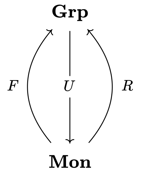
$R$이 $U$보다 더 파괴적이기 때문에 $U \dashv R$인 것으로 이해할 수 있다.

An Intuitive Understanding of Adjoints

16 Dec 2024

One of the central concepts in category theory is that of an adjoint.

Definition. Let $\mathcal{A}, \mathcal{B}$ be categories, and let $F: \mathcal{A} \to \mathcal{B}, G: \mathcal{B} \to \mathcal{A}$ be functors. We say that $F$ is a left adjoint to $G$, written as $F \dashv G$, if for any $A \in \mathcal{A}, B \in \mathcal{B}$, there exists a natural correspondence between $\hom_\mathcal{B}(F(A), B)$ and $\hom_\mathcal{A}(A, G(B))$. That is,

\[\begin{gather} (F(A) \xrightarrow{g} B) \quad \mapsto \quad (A \xrightarrow{\bar{g}} G(B))\\ (A \xrightarrow{f} G(B)) \quad \mapsto \quad (F(A) \xrightarrow{\bar{f}} B) \end{gather}\]

We also call $G$ the right adjoint to $F$.

This may feel very abstract, but there is a couple of examples that could be of assist in grasping the definition.

1. Adjoints as Approximations

When $F \dashv G$, the functors $F$ and $G$ can be thought of as approximating objects in $\mathcal{A}$ and $\mathcal{B}$ with respect to each other. In particular, the left adjoint represents approximation ‘from left to right’, while the right adjoint represents approximation ‘from right to left’.

For example, let $\mathbf{Z}$ be a category whose objects are integers, with a unique morphism $x \to y$ existing if and only if $x \leq y$. Similarly, let $\mathbf{R}$ be a category whose objects are real numbers, with a unique morphism $x \to y$ existing if and only if $x \leq y$. We may think of $\lceil \cdot \rceil, \lfloor \cdot \rfloor$ as functors $\mathbf{R} → \mathbf{Z}$, and the inclusion map $\iota$ as a functor $\mathbf{Z} → \mathbf{R}$. It then follows that $\lceil \cdot \rceil \dashv \iota \dashv \lfloor \cdot \rfloor$.

That is, $\lceil \cdot \rceil$ is a transformation that ‘lifts [a number] from left to right’ by mapping $r$ to $\lceil r \rceil$ with $r \leq \lceil r \rceil$, while $\lfloor \cdot \rfloor$ is a transformation that ‘pulls [a number] from right to left’ by mapping $r$ to $\lfloor r \rfloor$ with $\lfloor r \rfloor \leq r$.

Furthermore, let $I$ and $T$ be the initial object and terminal object of $\mathcal{A}$ respectively. That is, for any $A \in \mathcal{A}$:

• There exists a unique morphism $I \to A$.
• There exists a unique morphism $A \to T$.

For instance, in $\mathbf{Set}$, the empty set is the initial object and any singleton set is a terminal object.

For the singleton category $\mathcal{S}$, there exists a unique functor $F: \mathcal{A} \to \mathcal{S}$ that maps every object of $\mathcal{A}$ to the single object of $\mathcal{S}$. Let $G_I, G_T: \mathcal{S} \to \mathcal{A}$ be functors that maps the single object of $\mathcal{S}$ to $I$ and $T$, respectively. It then follows that $G_T \dashv F \dashv G_I$. (Since the terminal object is the ‘rightmost’ object, $G_T$ represents approximation ‘from left to right’, while since the initial object is the ‘leftmost’ object, $G_I$ represents approximation ‘from right to left’.)

2. Adjoints as Construction and Destruction

Left adjoints are associated with construction, while right adjoints are associated with destruction. Therefore, free functors are generally left adjoints, while forgetful functors are right adjoints.

For instance, let $\mathbf{Grp}$ be the category of groups and $\mathbf{Mon}$ be the category of monoids. Let $F$ be the free functor and $U$ be the forgetful functor. Define $R: \mathbf{Mon} → \mathbf{Grp}$ as follows:

• $R(M) = \lbrace m \in M : \exists m^{-1} \in M \rbrace$
• $R(f): m \mapsto f(m)$

Then the following diagram holds, yielding $F \dashv U \dashv R$.

One can understand $U \dashv R$ as expressing that $R$ is more destructive than $U$.

굴림에 대한 두 가지 삽화

11 Dec 2024

학부 시절 고전역학 수강 때 개인 공부용으로 만든 삽화인데, 잘 정리한 듯하여 이곳에도 공유한다.

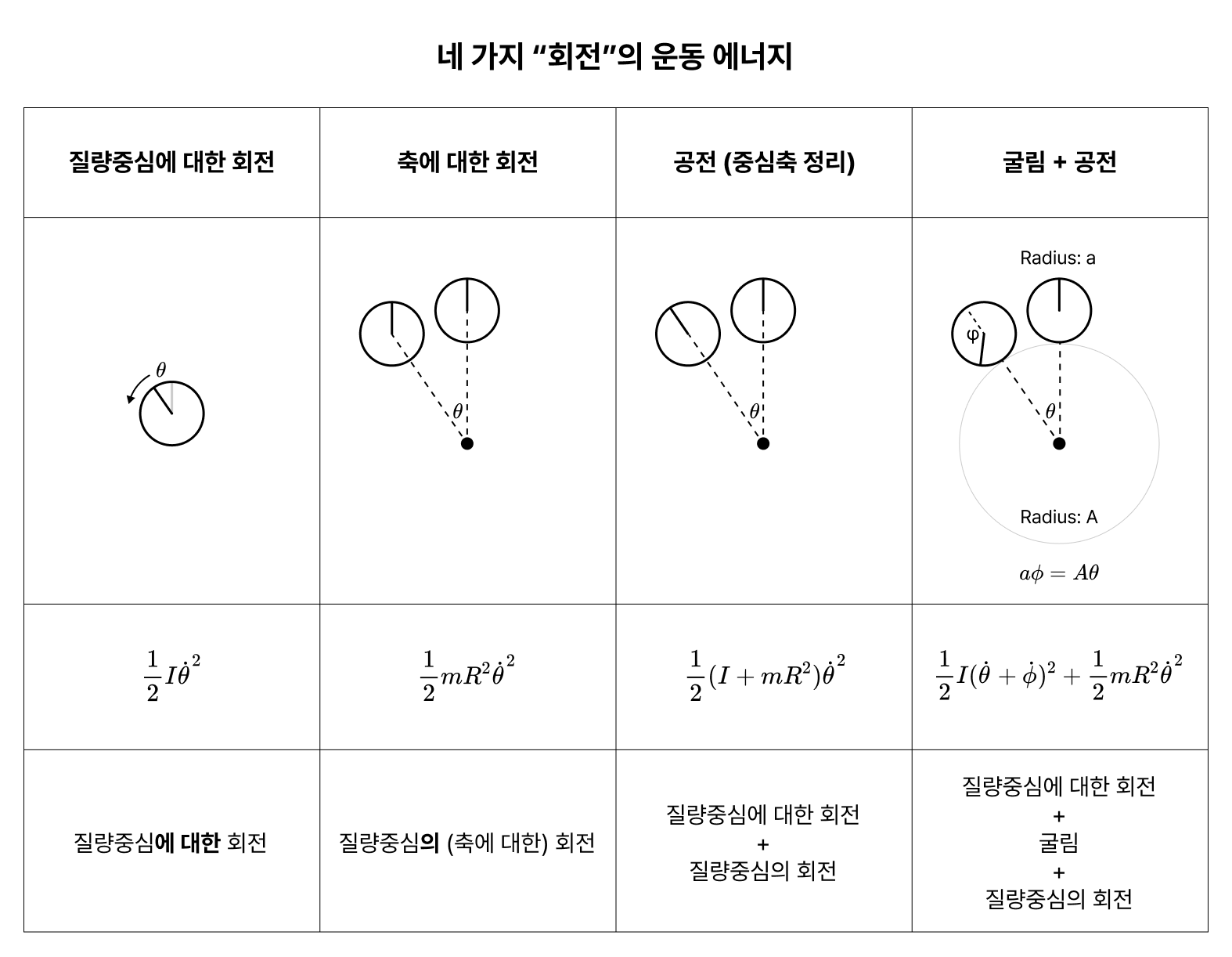
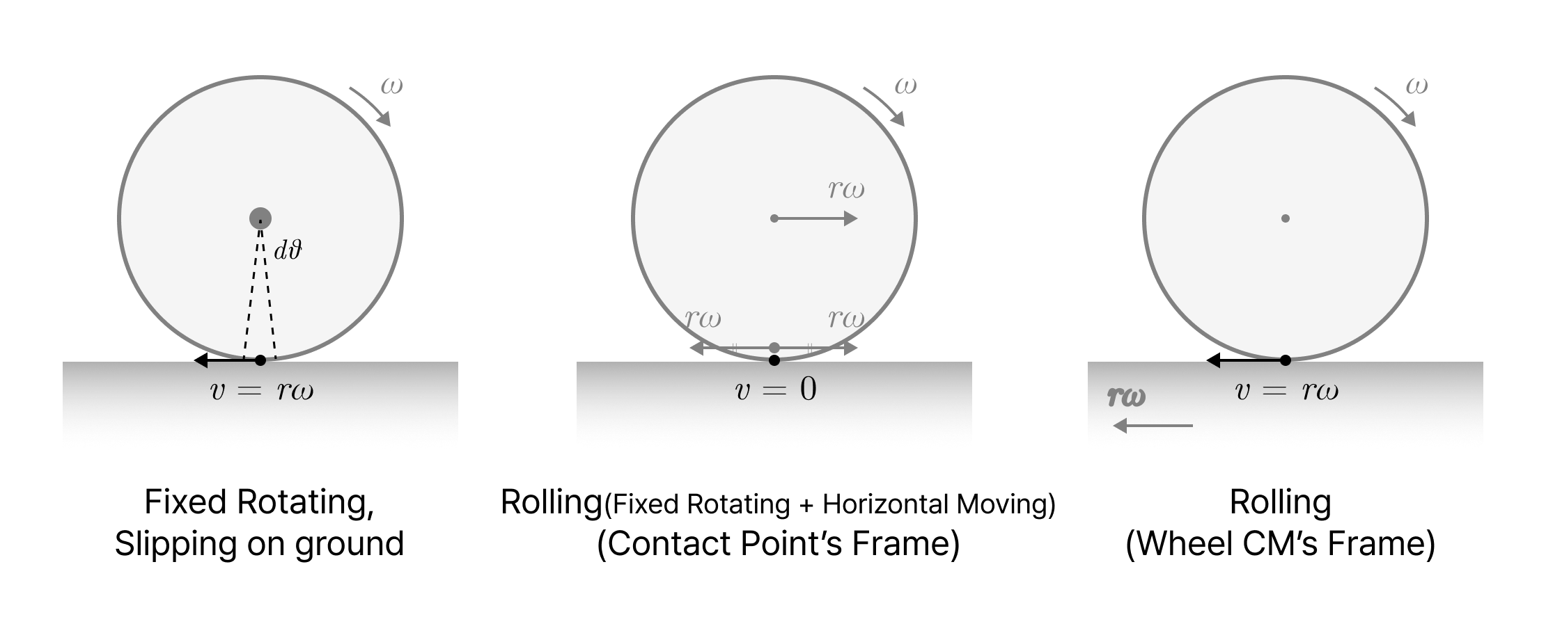
굴림을 바퀴의 CM 기준으로 분석할 때 땅 또한 움직인다는 사실에 유의하자.

Two Illustrations on Rolling

11 Dec 2024

These are illustrations I made when I studied classical mechanics in my BA. They seem to be well-made, so I decided to share them here, too.

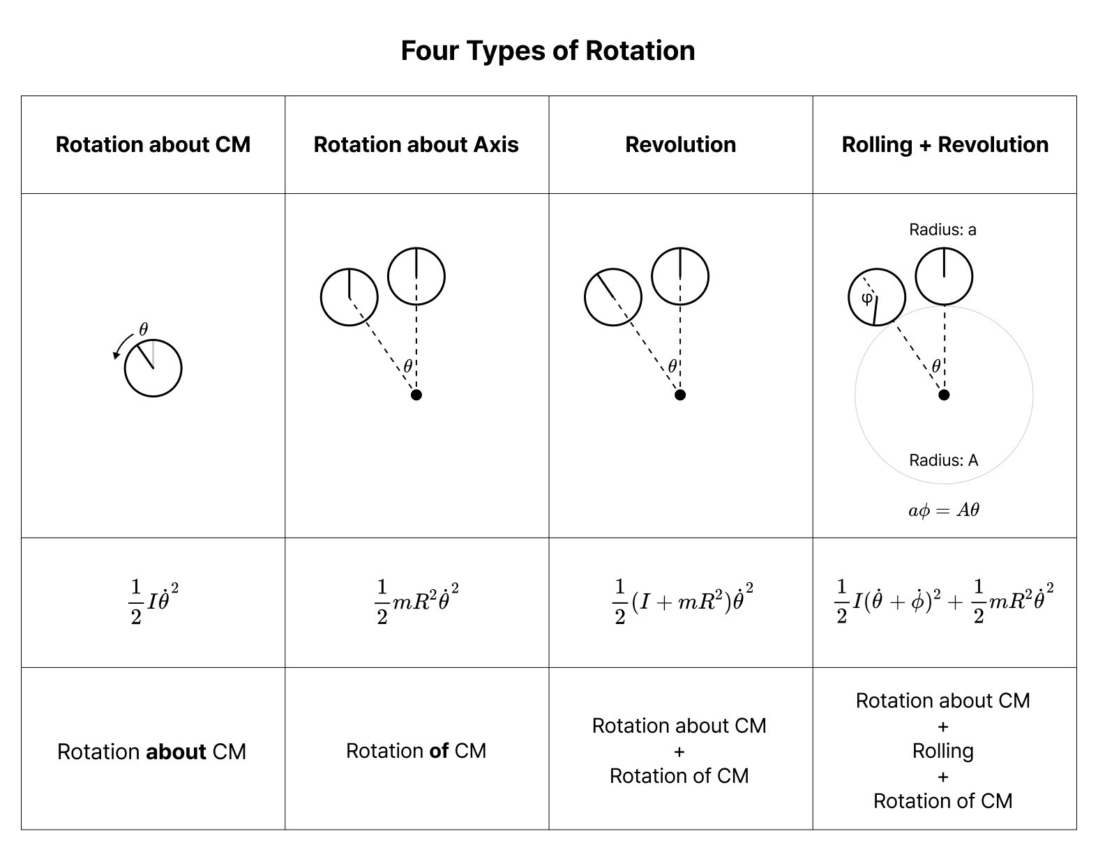
Note that decomposing Revolution as the sum of Rotation about CM and Rotation about Axis is a specific case of the central axis theorem.

Note that when analysing Rolling from CM’s frame, the ground also moves at $v = -r\omega$.

V = L 공리의 무모순성

11 Dec 2024

1. 전체

1.1. 폰 노이만 전체

초한귀납적으로 $\lbrace V_\alpha \rbrace$를 정의하자.

• $V_0 = \varnothing$
• $V_{\alpha + 1} = V_\alpha \cup \mathcal{P}(V_\alpha)$
• $\lambda$가 극한 서수일 때, $V_\lambda = \bigcup_{\alpha < \lambda} V_\alpha$

처음 몇 개의 $V_\alpha$는 다음과 같다.

• $V_1 = \lbrace \varnothing \rbrace$
• $V_2 = \lbrace \varnothing, \lbrace \varnothing \rbrace \rbrace$
• $V_3 = \lbrace \varnothing, \lbrace \varnothing \rbrace, \lbrace \lbrace \varnothing \rbrace \rbrace, \lbrace \varnothing, \lbrace \lbrace \varnothing\rbrace \rbrace \rbrace$
• $V_\omega = \mathsf{HF}$

모든 서수 $\alpha$에 대해 $V_\alpha$를 모아둔 모임을 폰 노이만 전체라고 한다.

\[V = \bigcup_{\alpha \in \mathrm{Ord}} V_\alpha\]

$x \in y \in z$가 $x \in z$를 시사할 때 $z$를 추이적 집합_{transitive set}이라고 한다. 이것은 $V$의 중요한 특징이다.

정리.

1. $\alpha \in \mathrm{Ord}$에 대해 $V_\alpha$는 추이적이다.
2. $V$는 추이적이다.

증명은 초한귀납법을 이용한다. 이에 따라 $V$를 다음과 같이 정의해도 무방하다.

• $V_0 = \varnothing$
• $V_{\alpha + 1} = \mathcal{P}(V_\alpha)$
• $\lambda$가 극한 서수일 때, $V_\lambda = \bigcup_{\alpha < \lambda}V_\alpha$

직관적으로 생각했을 때 $V$는 모든 집합을 포함하는 듯하다. 실제로 다음을 증명할 수 있다.

정리. $x$가 집합이라면 $x \in V$이다.

증명. 집합 $x$에 대해 $x$의 추이적 폐포 $\bar{x}$를, $x$를 원소로 가지는 가장 작은 추이적 집합으로 정의한다(이것이 well-defined임을 증명하기 위해서는 $x_0 = x, x_{n + 1} = \lbrace y : y \in x \text{ for some } x \in x_n \rbrace $일 때 $\bigcup x_n$가 $\bar{x}$임을 보이면 된다.)

$x \notin V$라고 가정하자. 분류 공리에 의해 $y = \lbrace u \in \bar{x} : u \notin V \rbrace$가 집합이며, 정초 공리에 의해 $y$의 $\in$-극소 원소 $z$가 존재한다. 만약 $w \notin V$인 $w \in z$가 존재한다면, 추이성에 의해 $w \in y$가 되어 $z$의 $\in$-극소성과 모순된다. 따라서 $z$의 모든 원소는 $V$에 있으며, 치환 공리로부터 $\Omega = \lbrace \alpha \in \mathrm{Ord} \mid \exists w \in z : w \in V_\alpha\rbrace$가 집합이다. $\beta = \bigcup_{\alpha \in \Omega}\alpha$라고 하자. $\beta$는 서수이며, $z \in V_{\beta + 1}$이다. (이 부분에서 $V_{\beta + 1} = \mathcal{P}(V_\beta)$임이 필요하다) 따라서 모순이다. ■

이에 따라 $V$는 집합이 아니다. 따라서 $V$는 모든 집합을 포함한다는 점에서 ZFC의 모델이지만, 많은 수학자들은 모델이 집합일 것을 요구하기 때문에 엄격한 의미에서의 모델은 아니다. 나중에 드러나겠지만, 이는 $V = L$의 무모순성 증명이 괴델의 제2불완전성 정리와 상충하지 않는 이유를 설명한다.

한편 $x \in V$는 “$x$는 집합이다“의 형식적 표현으로 이해하도록 한다.

1.2. 괴델 구성 가능 전체

먼저 다음과 같이 구성 가능성을 정의한다.

정의. 집합론의 언어를 $\mathcal{L}$이라고 하자. $X$가 $\mathcal{L}$-구조 $(L, \in)$에서 구성 가능하다는 것은, 어떤 $\mathcal{L}$-명제 $\phi$와 자유변수 할당 $g$가 존재하여 다음이 성립한다는 것이다.

\[X = \{ x \in L : (L, \in) \vDash \phi[g^0_x] \}\]

예를 들어 $L = \lbrace 0, 1, 2\rbrace$일 때 다음은 $X = \lbrace 1, 2 \rbrace$를 구성한다.

• $\phi(v_0, v_1, v_2) := (v_0 = v_1) \lor (v_0 = v_2)$
• $g: v_1 \mapsto 1, v_2 \mapsto 2$

또한 $L = \mathbb{N}$일 때 다음은 $X = \lbrace 0, 3, 6, 9, \dots \rbrace$를 구성한다.

• $\phi(v_0, v_1) := v_1 \mid v_0$
• $g: v_1 \mapsto 3$

괴델의 구성가능성은 언어로서의 표현가능성과 다르다. 일례로 언어로 표현가능한 실수의 집합은 가산이므로, 어떤 실수는 언어로 표현이 불가능하다. 그러한 실수를 $r$이라고 하자. $(L, \in)$이 실수 집합을 포함하는 구조일 때, 다음은 $X = \lbrace r \rbrace$을 구성한다.

• $\phi(v_0, v_1) := v_0 = v_1$
• $g: v_1 \mapsto r$

즉, 괴델의 구성가능성은 자유변수의 초기화를 임의의 원소에 대해 허용한다는 점에서 강력하다. 그러나 자유변수의 수가 유한하다는 점에서 한계를 가진다. 이제 초한귀납적으로 $\lbrace L_\alpha \rbrace$를 정의하자.

• $L_0 = \varnothing$
• $L_{\alpha + 1} = \lbrace x : x \text{ is constructible from } (L_\alpha, \in) \rbrace$
• $\lambda$가 극한 서수일 때, $L_\lambda = \bigcup_{\alpha < \lambda} L_\alpha$
• $L = \bigcup_{\alpha \in \mathrm{Ord}} L_\alpha$

$\alpha < \omega$일 때 $L_\alpha = V_\alpha$임을 쉽게 보일 수 있다. $\alpha = n$일 때, 최대 $n$개의 $\lor$ 연언으로 $x \in V_\alpha$를 구성할 수 있기 때문이다. 따라서,

• $L_1 = \lbrace \varnothing \rbrace$
• $L_2 = \lbrace \varnothing, \lbrace \varnothing \rbrace \rbrace$
• $L_3 = \lbrace \varnothing, \lbrace \varnothing \rbrace, \lbrace \lbrace \varnothing \rbrace \rbrace, \lbrace \varnothing, \lbrace \lbrace \varnothing\rbrace \rbrace \rbrace$
• $L_\omega = \mathsf{HF}$

하지만 $L_{\omega + 1} \subsetneq V_{\omega + 1}$이다. $\mathcal{P}(\mathbb{N}) \subset V_{\omega + 1}$이므로 $V_{\omega + 1}$은 비가산인 반면, 1차 논리 문장들의 집합과 $L_\omega$는 모두 가산이므로 $L_{\omega + 1}$ 또한 가산이기 때문이다. 일반적으로 $\alpha$가 가산일 때 $L_\alpha$는 가산이다.

그럼에도 $L$은 $V$와 많은 특징을 공유한다. 일례로,

정리. $\alpha \in \mathrm{Ord}$에 대해 다음이 성립한다.

1. $L_\alpha$는 추이적이다. (따라서 $L$이 추이적이다)
2. $\alpha \in L_{\alpha + 1} \setminus L_{\alpha}$

증명은 초한귀납법을 사용한다.

$L$은 모든 서수를 포함하므로 부랄리포르티 정리에 의해 집합이 아님에 유의하라. 대신 $x \in L_\alpha$에 대응되는 1차 논리식 $\mathsf{IsInL}_\alpha(x)$가 존재한다. 증명은 조금 까다로운데, 괴델 수를 이용하여 명제를 산술화하면 된다. (링크 참조) 따라서 $x \in L$을 $\exists \alpha \in \mathrm{Ord} :\mathsf{IsInL}_\alpha(x)$를 대체하는 형식적 표현으로 이해하여 사용하도록 한다. (물론 $\alpha \in \mathrm{Ord}$ 또한 1차 논리식을 대체하는 형식적 표현으로 이해되어야 한다)

2. 상대화

2.1. 명제의 상대화

1차 논리 명제는 양화사를 포함할 수 있다. 때문에 양화사의 정의역을 어떻게 설정하느냐의 따라 명제의 의미가 달라진다.

명제 $\phi$와 집합 (또는 모임) $A$에 대해, $\phi$의 상대화 $\phi^A$를 $\phi$의 모든 양화사를 $A$로 제한한 명제로 정의한다. 약간의 서사적 표현을 곁들이자면, $\phi^A$는 $A$의 “내부”에서 이해한 $\phi$라고 할 수 있겠다. 예를 들어, $\phi : \forall x \; \exists y : y < x$일 때

• $\phi^\mathbb{N} : \forall x \in \mathbb{N} \; \exists y \in \mathbb{N} : y < x$
• $\phi^\mathbb{Z} : \forall x \in \mathbb{Z} \; \exists y \in \mathbb{Z} : y < x$

$T_\mathbb{Q}$가 자연수 및 정수를 특정할 수 있는 정도의 표현력을 지니는 유리수 이론이라고 하면,

• $T_\mathbb{Q} \vdash \phi$
• $T_\mathbb{Q} \not\vdash \phi^\mathbb{N}$
• $T_\mathbb{Q} \vdash \phi^{\mathbb{Z}}$

이다. 따라서 $\phi$는 자연수와 유리수를 성공적으로 구분해 내지만, 정수와 유리수는 구분해 내지 못한다. 이 관찰을 일반화하면, 이론 $T$와 집합 $A$에 대해 $T \vdash \phi \leftrightarrow \phi^A$인 $\phi$가 많으면 많을수록 $A$는 $T$의 기술에 잘 “부합한다“고 말할 수 있다.

위 논의를 조금 일반화하여, 다음과 같이 정의한다.

정의. 이론 $T$와 집합 $A$에 대해서

\[T \vdash \forall x_1, \dots, x_n \in A (\phi(x_1, \dots, x_n) \leftrightarrow \phi^A(x_1, \dots, x_n))\]

일 때, $\phi$는 $A$에 대해 절대적_absolute이라고 한다.

일례로 $T_\mathbb{Q}$에 대해 $\phi(x) : \exists y (y < x)$는 정수에 대해 절대적이지만 자연수에 대해 절대적이지는 않다.

2.2. $L$-상대화

이제 우리의 목표는 $L$이 $\mathsf{ZF}$와 극대적으로 부합함을 보이는 것이다. 즉,

정리 1. $\phi$가 ZF의 공리라면 $\mathsf{ZF} \vdash \phi^L$이다.

정리 1의 의미를 말로 풀어 보자면,

“$L$의 내부에서 보았을 때 $L$은 ZF의 모델이다”를 ZF로 증명할 수 있다.

물론 우리는 $L \subset V$만 알고 $V = L$인지는 알지 못하기 때문에, 어떤 집합 $x$는 $L$에 속하지 않을 수도 있다. 그러나 설령 $x \in V \setminus L$인 집합 $x$가 있더라도, 그러한 $x$의 결여는 $L$의 내적 정합성을 깨뜨리지 않는다는 것이 정리 1의 내용이다.

예를 들어 어떤 집합 $y, z$에 대해 $x = \lbrace y, z \rbrace$가 $L$에 결여되어 있다고 하자. 일면 $x$의 결여는 $L$이 짝 공리 $\mathsf{Pair}$을 만족하지 않음을 시사하는 듯하다.

\[\mathsf{Pair} := \forall y, z \; \exists x \; \forall w: w \in x \leftrightarrow (w = y \lor w = z)\]

하지만 $L$의 내부에서 본 짝 공리는 다음과 같다.

\[\mathsf{Pair}^L := \forall y, z \in L \; \exists x \in L \; \forall w \in L: w \in x \leftrightarrow (w = y \lor w = z)\]

$\forall y, z$의 양화 또한 $L$로 한정됨에 주목하라. 즉, $x = \lbrace y, z \rbrace$의 결여가 $L$에게 문제를 일으키는 경우는 $y, z \in L$일 때이다. 거꾸로 말해, $x = \lbrace y, z \rbrace \notin L$이 $y, z \notin L$을 시사한다면 $L$은 $\mathsf{Pair}^L$을 만족한다. 이것이 “$L$이 내적 정합성을 유지하는 방식으로 집합을 결여한다”의 의미이다.

정리 1이 성립하는 핵심 이유는 $L$과 $V$가 추이성이라는 성질을 공유하기 때문이다.

보조정리. 다음 술어는 ZF에서 $L$에 대해 절대적이다.

1. $x \in y$
2. $x \subset y$
3. $x = \bigcup y$
4. $x = \lbrace y, z \rbrace$
5. $\alpha \in \mathrm{Ord}$
6. $x$는 추이적이다.
7. $\Delta_0$ 논리식

또한 다음을 증명할 수 있다.

정리 2. $\mathsf{ZF} \vdash (V = L)^L$

여기서 $V = L$은, “모든 집합이 $L$에 속한다”를 의미한다. 따라서 일면 보기에 $(V = L)^L$은 “$L$에 속하는 모든 집합이 $L$에 속한다”라는 자명한 명제인 듯하다. 하지만 실제로 $V = L$을 논리식으로 적으면

\[\forall x \; \exists \alpha : \alpha \in \mathrm{Ord} \land x \in L_\alpha\]

이므로 $(V = L)^L$은

\[\forall x \in L \; \exists \alpha \in L : (\alpha \in \mathrm{Ord})^L \land (x \in L_\alpha)^L\]

이다. 특히, $\alpha \in \mathrm{Ord}$와 $x \in L_\alpha$가 진정한 의미에서의 $\in$-술어가 아닌 1차 논리식의 형식적 표현이기 때문에 마찬가지로 $L$로 상대화해야 함에 유의하라. 이에 따라 $(V = L)^L$을 ZF에서 증명하기 위해서는 $\alpha \in \mathsf{Ord}$와 $x \in L_\alpha$가 절대적임을 증명해야 한다. 두 증명 모두 초한귀납법을 사용하면 가능하다.

정리 1과 정리 2로부터 다음을 증명할 수 있다.

정리 3. $\mathsf{ZFL} \vdash \phi \implies \mathsf{ZF} \vdash \phi^L$

증명. $\mathsf{ZFL} \vdash \phi$의 증명 길이에 대한 귀납법으로 증명한다. 증명 길이가 0일 때 $\phi$는 ZFL의 공리이다. $\phi$가 ZF의 공리일 때 정리 1로부터 증명되고, $\phi$가 $V = L$일 때 정리 2로부터 증명된다.

이제 $\phi$가 $\lbrace \psi_1, \dots, \psi_n \rbrace$에 추론 규칙을 적용하는 것으로 증명된다고 가정하자. $\psi_k$의 증명 길이는 $\phi$보다 작으므로 귀납 가정에 의해 $\mathsf{ZF} \vdash \psi_k^L$이며, 논리 공리와 추론 규칙은 $L$에 대해 절대적임을 쉽게 보일 수 있다. 따라서 $(\psi_1 \land \dots \land \psi_n) \rightarrow \phi$가 논리적 참이라면 $(\psi_1^L \land \dots \land \psi_n^L) → \phi^L$ 또한 논리적 참이며, 이에 따라 $\mathsf{ZF} \vdash \phi^L$이다. ■

정리 3의 따름정리로서 정리 4를 얻는다.

정리 4. ZF가 무모순적이라면 ZFL 또한 무모순적이다.

증명. ZFL이 모순적이라면 $\mathsf{ZFL} \vdash \varnothing \neq \varnothing$이며, 정리 3에 의해 $\mathsf{ZF} \vdash (\varnothing \neq \varnothing)^L \iff \mathsf{ZF} \vdash \varnothing \neq \varnothing$이다.

따라서 V = L은 ZF와 일관적이다.

Consistency of the V = L Axiom

11 Dec 2024

1. Universe

1.1. Von Neumann Universe

We define $\lbrace V_\alpha \rbrace$ using transfinite recursion.

• $V_0 = \varnothing$
• $V_{\alpha + 1} = V_\alpha \cup \mathcal{P}(V_\alpha)$
• When $\lambda$ is a limit ordinal, $V_\lambda = \bigcup_{\alpha < \lambda} V_\alpha$

The first few $V_\alpha$ are as follows:

• $V_1 = \lbrace \varnothing \rbrace$
• $V_2 = \lbrace \varnothing, \lbrace \varnothing \rbrace \rbrace$
• $V_3 = \lbrace \varnothing, \lbrace \varnothing \rbrace, \lbrace \lbrace \varnothing \rbrace \rbrace, \lbrace \varnothing, \lbrace \lbrace \varnothing\rbrace \rbrace \rbrace$
• $V_\omega = \mathsf{HF}$

The collection of all $V_\alpha$ for every ordinal $\alpha$ is called the Von Neumann universe.

\[V = \bigcup_{\alpha \in \mathrm{Ord}} V_\alpha\]

When $x \in y \in z$ implies $x \in z$, we call $z$ a transitive set. This is an important property of $V$.

Theorem.

1. For $\alpha \in \mathrm{Ord}$, $V_\alpha$ is transitive.
2. $V$ is transitive.

Proof. By transfinite induction.

Accordingly, we can also define $V$ as follows:

• $V_0 = \varnothing$
• $V_{\alpha + 1} = \mathcal{P}(V_\alpha)$
• When $\lambda$ is a limit ordinal, $V_\lambda = \bigcup_{\alpha < \lambda}V_\alpha$

Intuitively, $V$ appears to contain all sets. Indeed, we can prove the following:

Theorem. If $x$ is a set, then $x \in V$.

Proof. For a set $x$, we define the transitive closure $\bar{x}$ of $x$ as the smallest transitive set containing $x$ as an element. Note that this is well-defined as the intersection of transitive sets is transitive.

Assume $x \notin V$. By the axiom of separation, $y = \lbrace u \in \bar{x} : u \notin V \rbrace$ is a set, and by the axiom of foundation, there exists an $\in$-minimal element $z$ of $y$. If there exists $w \in z$ such that $w \notin V$, then by transitivity $w \in y$, contradicting the $\in$-minimality of $z$. Therefore, all elements of $z$ are in $V$, and by the axiom of replacement, $\Omega = \lbrace \alpha \in \mathrm{Ord} \mid \exists w \in z : w \in V_\alpha\rbrace$ is a set. Let $\beta = \bigcup_{\alpha \in \Omega}\alpha$. Then $\beta$ is an ordinal, and $z \in V_{\beta + 1}$. (This is where the definition of von Neumann universe $V_{\beta + 1} = \mathcal{P}(V_\beta)$ is invoked.) This yields a contradiction. ■

Consequently, $V$ is not a set. Therefore, while $V$ is a model of ZFC in the sense that it contains all sets, many mathematicians require models to be sets, so it is not a model in the strict sense. (This explains why our proof that $V$ is a ‘model’ of ZFC does not contradict Gödel’s incompleteness theorems; within ZFC, $V$ is not recognised as a valid set-theoretic object.) However, for convenience, in this article, we shall refer to $V$ as a model of set theory. Moreover, we shall understand $x \in V$ as a formal expression for “$x$ is a set”.

1.2. Gödel Constructible Universe

First, we define constructibility as follows:

Definition. Let $\mathfrak{A}$ be an $\mathcal{L}$-structure and let $A$ be the underlying domain of $\mathfrak{A}$. $u$ is constructible from $\mathfrak{A}$ if there exist some $\mathcal{L}$-formula $\phi(y, x_1, \dots, x_n)$ and $a_1, \dots, a_n \in A$ such that the following holds:

\[y \in u \iff y \in A \land \mathfrak{A} \vDash \phi(y, a_1, \dots, a_n)\]

Sometimes we abuse the notation and say that $u$ is constructible from $A$.

For example, with respect to the standard model of arithmetics, the following constructs $u = \lbrace 1, 2 \rbrace$:

• $\phi(y, x_1, x_2) : (y = x_1) \lor (y = x_2)$
• $a_1 = 1, a_2 = 2$

The following constructs $u = \lbrace 2, 5, 10, 17, \dots \rbrace$:

• $\phi(y, x_1) : \exists z (z \cdot z + x_1 = y)$
• $a_1 = 1$

Gödel’s constructibility differs from constructibility in the general sense, namely expressibility in language. For instance, since the set of real numbers expressible in language is countable, some real numbers cannot be expressed in language. Let such a real number be $r$. With respect to the standard model of real numbers, the following “constructs” $u = \lbrace r \rbrace$:

• $\phi(y, x_1) : x_1 = y$
• $a_1 = r$

That is, Gödel’s constructibility is more versatile than linguistic constructibility in that it allows initialisation of free variables to arbitrary elements. Nonetheless, it is constrained to have only finite number of free variables.

We now define $\lbrace L_\alpha \rbrace$ using transfinite recursion:

• $L_0 = \varnothing$
• $L_{\alpha + 1} = \lbrace x : x \text{ is constructible from } L_\alpha \rbrace$
• When $\lambda$ is a limit ordinal, $L_\lambda = \bigcup_{\alpha < \lambda} L_\alpha$
• $L = \bigcup_{\alpha < \lambda} L_\alpha$

We can easily show that $L_\alpha = V_\alpha$ when $\alpha < \omega$. Specifically, when $\alpha = n$, we can construct $x \in V_\alpha$ with at most $n$ disjunctions. Therefore:

• $L_1 = \lbrace \varnothing \rbrace$
• $L_2 = \lbrace \varnothing, \lbrace \varnothing \rbrace \rbrace$
• $L_3 = \lbrace \varnothing, \lbrace \varnothing \rbrace, \lbrace \lbrace \varnothing \rbrace \rbrace, \lbrace \varnothing, \lbrace \lbrace \varnothing\rbrace \rbrace \rbrace$
• $L_\omega = \mathsf{HF}$

However, $L_{\omega + 1} \subsetneq V_{\omega + 1}$. This is because although $\mathcal{P}(\mathbb{N}) \subset V_{\omega + 1}$ is uncountable, since the set of first-order logical sentences and $L_\omega$ are both countable, $L_{\omega + 1}$ is countable. In general, when $\alpha$ is countable, $L_\alpha$ is countable.

Nevertheless, $L$ shares many properties with $V$. For instance:

Theorem. For $\alpha \in \mathrm{Ord}$, the following hold:

1. $L_\alpha$ is transitive. (Therefore $L$ is transitive)
2. $\alpha \in L_{\alpha + 1} \setminus L_{\alpha}$

Proof. By transfinite induction.

Note that $L$ is not a set since it contains all ordinals. However, there exists a first-order formula $\mathsf{IsInL}_\alpha(x)$ that expresses $x \in L_\alpha$. The proof is intricate and involves arithmetising propositions using Gödel numbers. (See link) At any rate, this means that we may understand $x \in L$ as a formal expression expressing $\exists \alpha \in \mathrm{Ord} :\mathsf{IsInL}_\alpha(x)$. The two will be co-extensional for models of ZF.

2. Relativisation

2.1. Relativisation of Formulas

Definition. Let $T$ be an $\mathcal{L}$-theory and $\psi$ an $\mathcal{L}$-formula. We define the relativisation $\phi^\psi$, read as the relativisaion of $\phi$ respect to $\psi$, as the formula where all quantifiers in $\phi$ are restricted to satisfy $\psi$.

Using $\mathsf{PA}$ as an example, if $\psi(x) : \exists z(z + z = x)$ and $\phi(x) : \exists z(z \cdot z = x)$, then:

\[\phi^\psi(x) : \exists z (\psi(z) \land z \cdot z = x)\]

Semantically, $\phi(x)$ expresses “$x$ is a perfect square” while $\phi^\psi(x)$ expresses “$x$ is a square of an even number”.

When it is clear that what $\psi(x)$ is supposed to express is $x \in S$, then we abuse the notation and write $\phi^S$ instead of $\phi^\psi$. Hence in the case of the previous example, we may write $\phi^E$ instead, where $E$ is the set of even numbers. That is,

\[\phi^E(x) : \exists z \in E (z \cdot z = x)\]

To use a bit of metaphoric expression, $\phi^S$ is how $\phi$ is “seen from” $S$.

For example, let $o(x)$ be the first-order formula expressing “$x$ is an ordinal”. Specifically, it is defined as:

\[o(x) : \mathrm{tr}(x) \land \forall y \in x \; \mathrm{tr}(y)\]

where $\mathrm{tr}(x) : \forall y \in x \; \forall z \in y (z \in x)$ expresses “$x$ is transitive”. By the abuse of notation, we may write $\phi^{\mathrm{Ord}}$ instead of $\phi^o$. $\phi^{\mathrm{Ord}}$ is how $\phi$ is “seen from” the class of all ordinals. Define:

• $\phi_1 : \forall x \exists y \forall z (z \subset x \rightarrow z \in y)$
• $\phi_2 : \forall x \forall y \exists z (z = x \cup y)$

That is, $\phi_1$ expresses closure under power set operation and $\phi_2$ expresses closure under set union. We have:

• $\mathsf{ZFC} \not\vdash \phi_1^\mathrm{Ord}$
• $\mathsf{ZFC} \vdash \phi_2^\mathrm{Ord}$,

since the set of ordinals is closed under union but not under power set. Put in another way, $\phi_1$ successfully distinguishes the class of all sets — what ZFC tries to describe — and the class of ordinals, while $\phi_2$ cannot. Generalising this observation, for a theory $T$ and a set $A$, the more formulas $\phi$ such that $T \vdash \phi \leftrightarrow \phi^A$, the better $A$ “conforms” to the description of $T$.

This leads us to the following definition.

Definition. For an $\mathcal{L}$-theory $T$ and a set $A$, $\phi$ is said to be absolute with respect to $A$ if for every $\mathcal{L}$-formula $\phi$,

\[T \vdash \forall x_1, \dots, x_n \in A (\phi(x_1, \dots, x_n) \leftrightarrow \phi^A(x_1, \dots, x_n))\]

Note that the definition simply becomes $T \vdash \phi^A$ when $\phi$ has no free variables, and it is given that $T \vdash \phi$.

2.2. $L$-Relativisation

Our goal now is to show that the axioms of ZF are absoulte with respect to $L$. That is:

Theorem 1. If $\phi$ is an axiom of ZF, then $\mathsf{ZF} \vdash \phi^L$.

That is to say,

“When seen from $L$, $L$ is a model of ZF” can be proved in ZF.

Of course, we only know that $L \subset V$ and do not know whether $V = L$, which leaves open the possibility of some set $x$ not belonging to $L$. Yet according to Theorem 1 states is that, even if there exists such a set $x$, its abscence does not break the internal consistency of $L$.

For example, suppose some set $x = \lbrace y, z \rbrace$ is absent from $L$. At first glance, the absence of $x$ seems to suggest that $L$ does not satisfy the pairing axiom $\mathsf{Pair}$:

\[\mathsf{Pair} := \forall y, z \; \exists x \; \forall w: w \in x \leftrightarrow (w = y \lor w = z)\]

However, the pairing axiom as viewed from inside $L$ is:

\[\mathsf{Pair}^L := \forall y, z \in L \; \exists x \in L \; \forall w \in L: w \in x \leftrightarrow (w = y \lor w = z)\]

Note that the quantification $\forall y, z$ is also restricted to $L$. That is, the absence of $x = \lbrace y, z \rbrace$ causes problems in $L$ only when $y, z \in L$. Conversely, if $x = \lbrace y, z \rbrace \notin L$ implies $y, z \notin L$, then $L$ satisfies $\mathsf{Pair}^L$. This is, $L$ lacks sets only in a way that maintains internal consistency.

Although we do not give the full proof, we highlight that the key reason Theorem 1 holds is that $L$, like $V$, is a transitivie class of sets, which leads to the following lemma.

Lemma. The following predicates are absolute with respect to $L$ in ZF:

1. $x \in y$
2. $x \subset y$
3. $x = \bigcup y$
4. $x = \lbrace y, z \rbrace$
5. $\alpha \in \mathrm{Ord}$
6. $x$ is transitive
7. $\Delta_0$ formulas

From this lemma, it is not too difficult to prove Theorem 1. Moreover, we can prove:

Theorem 2. $\mathsf{ZF} \vdash (V = L)^L$

Here, $V = L$ is a formal expression standing for $\forall x (x \in L)$. At first glance it may seem that $(V = L)^L$ is thus the trivial proposition $\forall x \in L (x \in L)$. However, when we actually expand $V = L$ as a first-order formula, we have:

\[\forall x \; \exists \alpha \; (\alpha \in \mathrm{Ord} \land x \in L_\alpha)\]

so $(V = L)^L$ becomes:

\[\forall x \in L \; \exists \alpha \in L \; (\alpha \in \mathrm{Ord})^L \land (x \in L_\alpha)^L\]

Note particularly that since $\alpha \in \mathrm{Ord}$ and $x \in L_\alpha$ are formal expressions of first-order formulas rather than a genuine $\in$-relation, they must likewise be relativised to $L$. Thus, to prove $(V = L)^L$ in ZF, we must prove that $\alpha \in \mathrm{Ord}$ and $x \in L_\alpha$ are also absolute. The former follows from the previous lemma, and the latter also “almost” follows from the lemma, except that $x \in L_\alpha$ is a $\Sigma_1$-sentence, so slightly more argument is required to secure its absoluteness.

From Theorems 1 and 2, we can prove:

Theorem 3. $\mathsf{ZFL} \vdash \phi \implies \mathsf{ZF} \vdash \phi^L$

Proof. We prove by induction on the proof length of $\mathsf{ZFL} \vdash \phi$. When the proof length is 0, $\phi$ is an axiom of ZFL. When $\phi$ is an axiom of ZF, it follows from Theorem 1, and when $\phi$ is $V = L$, it follows from Theorem 2.

Now assume $\phi$ is proved by applying an inference rule to $\lbrace \psi_1, \dots, \psi_n \rbrace$. The proof length of $\psi_k$ is smaller than that of $\phi$, so by the induction hypothesis $\mathsf{ZF} \vdash \psi_k^L$. We can easily show that logical axioms and inference rules are absolute with respect to $L$. Using modus ponens as an example, this means that:

\[\mathsf{ZF} \vdash ((\phi \land \phi \rightarrow \psi) \rightarrow \psi)^L\]

Therefore, if $(\psi_1 \land \dots \land \psi_n) \rightarrow \phi$ is logically valid, then $(\psi_1^L \land \dots \land \psi_n^L) → \phi^L$ is also logically valid, and consequently $\mathsf{ZF} \vdash \phi^L$. ■

As a corollary of Theorem 3, we obtain Theorem 4:

Theorem 4. If ZF is consistent, then ZFL is also consistent.

Proof. If ZFL is inconsistent, then $\mathsf{ZFL} \vdash \varnothing \neq \varnothing$, and by Theorem 3, $\mathsf{ZF} \vdash (\varnothing \neq \varnothing)^L \iff \mathsf{ZF} \vdash \varnothing \neq \varnothing$, which contradicts the consistency of ZF. ■

Therefore, V = L is consistent with ZF.

초한귀납과 초한재귀

05 Dec 2024

1. 초한귀납법

정리. $P$가 서수 위에서 정의된 속성이고 임의의 $\alpha \in \mathrm{Ord}$에 대해

\[[ \forall \beta < \alpha : P(\beta)] → P(\alpha)\]

가 성립할 때, $P$는 모든 서수에 대해 참이다.

Remark. $P$의 정의역인 $\mathrm{Ord}$는 집합이 아닌 진모임_{proper class}이므로 “술어” 대신 “속성”이란 표현을 사용한다.

증명. 서수가 정렬 순서라는 사실과 귀류법을 사용한다.

$\lnot P(\lambda)$인 $\lambda$가 존재한다고 하자. $\Omega = \lbrace \alpha \in \lambda : \lnot P(\alpha) \rbrace$는 공집합이 아닌 정렬 집합이므로 최소 원소 $\alpha_0$가 존재한다. 이때 $\forall \beta < \alpha_0 : P(\beta)$이므로 가정에 의해 $P(\alpha_0)$가 되어 모순이다. ■

응용. 폰 노인만 계층에서 $V_\alpha$는 추이적이다. 따라서 $V_{\alpha + 1} = V_\alpha \cup \mathcal{P}(V_\alpha)$ 대신 $V_{\alpha + 1} = \mathcal{P}(V_\alpha)$로 정의할 수 있다.

2. 초한재귀적 정의

Motivation. 자연수의 재귀적 정의를 생각해 보자. $n$개의 집합 $x_1, \dots , x_n$이 주어졌을 때 집합을 출력하는 함수 $g$가 존재한다면 다음과 같이 $f: \mathbb{N} → V$을 정의할 수 있을 것이다.

\[f(n) = g(f(0), \dots, f(n - 1))\]

문제는 $g$가 고정된 수의 매개변수만을 가질 수 있다는 것이다. 따라서 다음과 같이 $g$의 매개변수를 순서쌍으로 묶는다.

\[f(n) = g(\langle f(0), \dots, f(n - 1) \rangle)\]

이 순서쌍은 $\lbrace (0, f(0)), \dots, (n - 1, f(n - 1)) \rbrace = f \upharpoonright n$과 같이 표현할 수 있다. 즉,

\[f(n) = g(f \upharpoonright n).\]

이를 서수에 대해서 일반화하면 다음과 같다.

정리. $G: V → V$가 모임함수(class function)이라고 하자. 다음을 만족하는 모임함수 $F: \mathrm{Ord} → V$가 존재한다.

\[F(\alpha) = G(F \upharpoonright \alpha)\]

증명. 초한귀납법을 겁나게 쓰면 된다. (불친절해서 ㅈㅅ)