Construction of Measures via Carathéodory's Theorem

25 Feb 2025

I prefer to approach Carathéodory’s theorem by dividing it into three subtheorems. They are as follows:

1. Carathéodory Construction Theorem: Any collection of sets and a positive function define an outer measure.
2. Carathéodory Restriction Theorem: Restricting the domain of an outer measure to measurable sets yields a measure.
3. Carathéodory Extension Theorem: There exists a unique extension of premeasure $\mu_0$ on an algebra $\mathcal{A}_0$ to a measure $\mu$ on the $\sigma$-algebra $\sigma(\mathcal{A}_0)$. Furthermore, $\mu$ is the measure obtained by applying the construction theorem with the collection of sets as $\mathcal{A}_0$ and the positive function as $\mu_0$, and then applying the restriction theorem.

Schematically, this can be understood as follows:

	(1)	(2)	(3)
Domain	Algebra $\mathcal{A}_0$	$\sigma$-algebra $\mathcal{A}$	Power set $\mathcal{P}(X)$
Function	Premeasure $\mu_0$	Measure $\mu$	Outer measure $\mu^\ast$

The construction theorem goes in the direction (1) → (3), the restriction theorem goes (3) → (2), and the extension theorem goes (1) → (2). Let us examine each one by one.

Definition. An outer measure $\mu^\ast: \mathcal{P}(X) \to [0, \infty]$ on $X$ is a function satisfying the following:

1. $\mu^\ast(\varnothing) = 0$
2. $A \subset B \implies \mu^\ast(A) \leq \mu^\ast(B)$
3. $\mu^\ast\left( \bigcup_{n \in \mathbb{N}} A_n \right) \leq \sum_{n \in \mathbb{N}} \mu^\ast(A_n)$

Carathéodory Construction Theorem. Given any collection $\mathcal{S}$ of subsets of $X$ and any function $l: \mathcal{S} \to [0, \infty]$ satisfying $l(\varnothing) = 0$, the function $\mu^\ast$ defined as follows is an outer measure:

\[\mu^*(E) = \inf \left\{ \sum_{n \in \mathbb{N}} l(A_n) : \{ A_n \} \subset \mathcal{S} \text{ covers }E \right\}\]

That is, $\mu^\ast$ is a function that defines something akin to a ‘measure’ of $E$ as an infimum over covers, and is conceptually similar to the upper sum_{upper sum} in Riemann integration.

Proof. Properties 1 and 2 are trivial. We prove property 3.

Let $A = \bigcup A_n$ and suppose an arbitrary $\epsilon > 0$ is given. By the definition of $\mu^\ast$, for each $n$, there exists a cover $\mathcal{C}_n = \lbrace A_{nm} \rbrace_{m \in \mathbb{N}} \subset \mathcal{S}$ of $A_n$ satisfying:

\[\sum l(A_{nm}) \leq \mu^*(A_n) + \epsilon/2^n\]

Therefore,

\[\sum_{n, m \in \mathbb{N}} l(A_{nm}) \leq \sum \mu^*(A_n) + \epsilon.\]

Since $\bigcup \mathcal{C}_n$ covers $A$, by the definition of $\mu^\ast$, we have $\mu^\ast(A) \leq \sum_{n, m \in \mathbb{N}} l(A_{nm})$. ■

Definition. Let $\mu^\ast$ be an outer measure. A set $A$ is said to be measurable with respect to $\mu^\ast$ if it satisfies the following for any $E$:

\[\mu^*(E) = \mu^*(E \cap A) + \mu^*(E \cap A^c)\]

Definition. Let $\mu^\ast$ be an outer measure. A set $N$ with $\mu^\ast(N) = 0$ is called a null set.

That is, a measurable set is one that ‘cleanly’ partitions any set with respect to $\mu^\ast$. Therefore, we can expect that $\mu^\ast$ will behave like an ordinary measure on the collection consisting only of measurable sets. The following restriction theorem validates this expectation.

Carathéodory Restriction Theorem. Let $\mu^\ast$ be an outer measure. Let $\mathcal{A}$ be the collection of sets that are measurable with respect to $\mu^\ast$. Then the following hold:

1. $\mathcal{A}$ is a $\sigma$-algebra.
2. $\mu^\ast |_\mathcal{A}$ is a measure.
3. $\mathcal{A}$ contains all null sets of $\mu^\ast$.

Proof.

1. $\mathcal{A}$ is an algebra.

Closure under complements is trivial. We show closure under finite intersections.

Suppose $A, B$ are measurable. To show that $A \cap B$ is measurable, it suffices to prove:

\[\mu^*(E \cap (A \cap B)) + \mu^*(E \cap (A \cap B)^c) \leq \mu^*(E) \quad \cdots \quad (*)\]

Since $A, B$ are measurable, the following holds:

\[\begin{aligned} \mu^*(E) &= \mu^*(E \cap A) + \mu^*(E \cap A^c) \\ &= \mu^*(E \cap A \cap B) + \mu^*(E \cap A \cap B^c) \\ &+ \mu^*(E \cap A^c \cap B) + \mu^*(E \cap A^c \cap B^c) \end{aligned}\]

Therefore, $(\ast)$ is equivalent to:

\[\begin{aligned} \mu^*(E \cap (A^c \cup B^c)) &\leq \mu^*(E \cap A \cap B^c) \\ &+ \mu^*(E \cap A^c \cap B) \quad \cdots \quad (**) \\ &+ \mu^*(E \cap A^c \cap B^c) \end{aligned}\]

From elementary set theory, we have:

\[A^c \cup B^c = (A \cap B^c) \cup (A^c \cap B) \cup (A^c \cap B^c)\]

Therefore, $(\ast\ast)$ holds. □

2. $\mathcal{A}$ is a $\sigma$-algebra.

It suffices to show that for $\lbrace A_n \rbrace \subset \mathcal{A}$ with $A_n \uparrow A$, we have $A \in \mathcal{A}$. (Why?)

By the definition of outer measure, $\mu^\ast(E \cap A_n) \leq \mu^\ast(E \cap A)$. Let $C_1 = A_1, C_n = A_n \setminus A_{n - 1}$. Then $\bigsqcup C_n = A$. Moreover,

\[\begin{aligned} \mu^*(E \cap A_n) &= \mu^*(E \cap A_n \cap C_n) + \mu^*(E \cap A_n \cap C_n^c) \\ &= \mu^*(E \cap C_n) + \mu^*(E \cap A_{n - 1}) \\ &= \cdots \\ &= \sum^n_{k = 1} \mu^*(E \cap C_k) \end{aligned}\]

Therefore, $\sum^\infty \mu^\ast(E \cap C_n) \leq \mu^\ast(E \cap A)$. Since $\lbrace E \cap C_n \rbrace $ covers $E \cap A$, we have $\sum^\infty \mu^\ast(E \cap C_n) \geq \mu^\ast(E \cap A)$. Therefore, $\sum^\infty \mu^\ast(E \cap C_n) = \mu^\ast(E \cap A)$.

Thus, for any $\epsilon > 0$, there exists a sufficiently large $N$ such that $\mu^\ast(E \cap A) - \epsilon \leq \mu^\ast(E \cap A_n)$. Therefore,

\[\begin{aligned} \mu^*(E \cap A_n^c) &= \mu^*(E) - \mu^*(E \cap A_n) \\ &\leq \mu^*(E) - \mu^*(E \cap A) + \epsilon \end{aligned}\]

whence we obtain:

\[\mu^*(E) \leq \mu^*(E \cap A_n) + \mu^*(E \cap A_n^c) \leq \mu^*(E) + \epsilon\]

Letting $n \to \infty$, we get $\mu^\ast(E \cap A) + \mu^\ast(E \cap A^c) = \mu^\ast(E)$. □

3. $\mu^\ast|_\mathcal{A}$ is a measure, 4. $\mathcal{A}$ contains all null sets.

Left as an exercise to the readers. (Not difficult) ■

Definition. Let $\mathcal{A}_0$ be an algebra. A function $\rho: \mathcal{A}_0 \to [0, \infty]$ is called a premeasure if it satisfies the following:

1. $\rho(\varnothing) = 0$
2. For any pairwise disjoint countable collection $\lbrace A_n \rbrace $, if $\bigcup A_n \in \mathcal{A}_0$, then $\rho\left( \bigcup A_n \right) = \sum \rho(A_n)$

Carathéodory Extension Theorem. For a premeasure $\rho$ on an algebra $\mathcal{A}_0$, define:

\[\mu^*(E) = \inf \left\{ \sum_{n \in \mathbb{N}} \mu_0(A_n) : \{ A_n \} \subset \mathcal{A}_0 \text{ covers }E \right\}\]

Then the following hold:

1. If $A \in \mathcal{A}_0$, then $\mu^\ast(A) = \rho(A)$.
2. $\sigma(\mathcal{A}_0)$ is measurable with respect to $\mu^\ast$.
3. If $\rho$ is $\sigma$-finite, then $\mu^\ast|_{\sigma(\mathcal{A}_0)}$ is the unique measure that extends $\rho$ to $\sigma(\mathcal{A}_0)$.

Proof.

1. If $A \in \mathcal{A}_0$, then $\mu^\ast(A) = \rho(A)$.

Since $A$ is a cover of $A$, we have $\mu^\ast(A) \leq \rho(A)$. If $\mu^\ast(A) < \rho(A)$, then there exists some cover $\lbrace A_n \rbrace $ of $A$ such that $\sum \rho(A_n) < \rho(A)$. However, since $\rho$ is a premeasure, this is a contradiction. □

2. $\sigma(\mathcal{A}_0)$ is measurable with respect to $\mu^\ast$.

First, we show that $\mathcal{A}_0$ is measurable. For any $A \in \mathcal{A}_0$, it suffices to show $\mu^\ast(E \cap A) + \mu^\ast(E \cap A^c) \leq \mu^\ast(E)$. By the definition of $\mu^\ast$, for any $\epsilon > 0$, there exists some cover $\mathcal{C}$ of $E$ such that:

\[\sum^\infty_{n = 1} \rho(C_n) \leq \mu^*(E) + \epsilon\]

Since $\mathcal{A}_0$ is an algebra, $A \cap C_n, A^c \cap C_n \in \mathcal{A}_0$. Therefore,

\[\begin{aligned} \mu^*(E \cap A) + \mu^*(E \cap A^c) &\leq \sum^\infty_{n = 1} \mu^*(A \cap C_n) + \sum^\infty_{n = 1} \mu^*(A^c \cap C_n) \\ &= \sum^\infty_{n = 1} \rho(A \cap C_n) + \sum^\infty_{n = 1} \rho(A^c \cap C_n) \\ &= \sum^\infty_{n = 1} \rho(C_n) \leq \mu^*(E) + \epsilon \end{aligned}\]

(Strictly speaking, one should consider $\sum^n_{k=1}$ and then take the limit $n \to \infty$) Therefore, $\mu^\ast(E \cap A) + \mu^\ast(E \cap A^c) \leq \mu^\ast(E)$, and $\mathcal{A}_0$ is measurable. By the Carathéodory restriction theorem, measurable sets form a $\sigma$-algebra, so $\sigma(\mathcal{A}_0)$ is also measurable. □

3. If $\rho$ is $\sigma$-finite, then $\mu^\ast|_{\sigma(\mathcal{A}_0)}$ is the unique measure that extends $\rho$ to $\sigma(\mathcal{A}_0)$.

First, assume $\rho < \infty$. Suppose a measure $\nu$ defined on $\sigma(\mathcal{A}_0)$ agrees with $\rho$ on $\mathcal{A}_0$. Let $\mu = \mu^\ast|_{\sigma(\mathcal{A}_0)}$. We show $\nu = \mu$.

Let $E \in \sigma(\mathcal{A}_0)$. There exists some cover $\lbrace A_n \rbrace \subset \mathcal{A}_0$ of $E$ such that:

\[\sum \rho(A_n) \leq \mu(E) + \epsilon\]

Since $\nu$ agrees with $\rho$ on $\mathcal{A}_0$, we have $\sum \rho(A_n) = \sum \nu(A_n) \geq \nu(E)$. Therefore, $\nu \leq \mu$.

Now define $B_n = \bigcup^n_{k=1}A_k$ and let $A = \bigcup^\infty_{n = 1} A_n = \lim_{n \to \infty} B_n$. Since $\mu(B) = \sum \rho(A_n) \leq \mu(E) + \epsilon$, we have $\mu(B \setminus E) \leq \epsilon$. Since $\nu$ is a measure,

\[\mu(A) = \lim \rho(B_n) = \lim \nu(B_n) = \nu(A)\]

Therefore,

\[\begin{aligned} \mu(E) \leq \mu(B) &= \mu(B \setminus E) + \mu(E) \\ &\leq \epsilon + \nu(E) \end{aligned}\]

That is, $\mu \leq \nu$. Therefore, $\mu = \nu$.

Now assume $\rho$ is $\sigma$-finite. There exists a collection $\lbrace C_n \rbrace $ such that $C_n \uparrow X$ and $\rho(C_n) < \infty$. By the preceding argument, $\mu$ and $\nu$ agree on $C_n$. Therefore,

\[\mu(A) = \lim \mu(A \cap C_i) = \lim \nu (A \cap C_i) = \nu(A)\]

so $\mu$ and $\nu$ agree on the entire space. ■

In the next article, we shall construct Lebesgue measure using Carathéodory’s theorem, and then show that while every Borel measurable set is Lebesgue measurable, the converse does not hold.

대수와 측도의 정의

24 Feb 2025

1. 비탈리 정리

정의. $\mu$가 집합 $X$ 위의 측도_measure라는 것은 다음을 만족한다는 것이다.

1. $\mu(\varnothing) = 0$
2. 쌍으로 서로소_{pairwise disjoint}인 가산 집합족 $\lbrace A_n \rbrace$에 대해, $\mu\left( \bigcup A_n \right) = \sum \mu(A_n)$

유감스럽게도 $X = \mathbb{R}$일 때, 측도 $\mu$는 실수의 모든 부분집합에 대해서 정의될 수 없다.

비탈리 정리. 다음을 모두 만족하는 $\mathbb{R}$의 측도 $\mu$는 존재하지 않는다.

1. 항등적으로 0이 아니다.
2. 평행이동에 대해 보존적이다. 즉, 임의의 $r \in \mathbb{R}$에 대해 $\mu(A + r) = \mu(A)$.
3. $\operatorname{dom} \mu = \mathcal{P}(\mathbb{R})$

증명. 그러한 측도 $\mu$가 존재한다고 가정하자. $\mathbb{R}$ 위에서 다음의 동치 관계를 정의하자.

\[x \sim y \iff x - y \in \mathbb{Q}\]

선택 공리에 의해 $[0, 1]/{\sim}$의 선택 함수 $\iota$가 존재한다. $V = \operatorname{im} \iota$라고 하자. $V$를 비탈리 집합_{Vitali set}이라고 부른다. 예를 들어 $V = \lbrace 0.1, \pi - 3, \sqrt{2} - 1, \dots \rbrace$이다. $\mu$는 $V$에서 정의될 수 없음을 보인다.

$V$의 정의에 의해, $q \in \mathbb{Q}$에 대해 $V$와 $V + q$는 서로소이다. 또한 $[0, 1] \subset \bigcup_{q \in \mathbb{Q}} (V + q) \subset [-1, 3]$이다. 따라서,

\[1 \leq \sum_{q \in \mathbb{Q}}\mu(V + q) \leq 4.\]

그런데 $\mu(V + q) = \mu(V)$이므로, $\mu(V) = 0$이면 왼쪽 부등식이 성립하지 않고 $\mu(V) > 0$이면 오른쪽 부등식이 성립하지 않는다. 따라서 모순이다. ■

2. $\sigma$-대수

따라서 올바른 측도를 구축하기 위해서는 측도의 정의역을 적절히 제한할 필요가 있다. 이에 대수의 개념을 도입한다.

정의. 집합 $X$의 대수_algebra $\mathcal{A}_0$는 다음을 만족하는 집합족이다.

1. $\varnothing, X \in \mathcal{A}_0$
2. $A \in \mathcal{A}_0 \implies A^c \in \mathcal{A}_0$
3. $A, B \in \mathcal{A}_0 \implies A \cup B \in \mathcal{A}_0$

Remark. 2번 공리와 드모르간의 법칙에 의해, 3번 공리는 $A \cap B \in \mathcal{A}_0$ 또한 시사한다.

대수의 3번 정의를 가산 합집합으로 강화하면 $\sigma$-대수의 정의를 얻는다. 즉,

정의. 집합 $X$의 $\sigma$-대수 $\mathcal{A}$는 다음을 만족하는 대수이다.

1. $\lbrace A_n \rbrace _{n \in \mathbb{N}} \subset \mathcal{A}_0 \implies \bigcup_{n \in \mathbb{N}} A_n \in \mathcal{A}$

정리. $\lbrace \mathcal{A}_i \rbrace_{i \in I}$가 $X$의 $\sigma$-대수들의 모임이라면 $\bigcap_{i \in I}\mathcal{A}_i$ 또한 $X$의 $\sigma$-대수이다.

증명. $\sigma$-대수의 정의로부터 쉽게 증명할 수 있다. 그런데 이렇게만 적으면 재미 없으니까, 조금 독특한 증명을 남긴다. 워시-타르스키 정리_{Łoś-Tarski theorem}에 따르면 1차 이론이 교집합에 대해 보존적일 필요충분조건은 1차 이론의 모든 문장이 $\Pi_1$ 문장인 것이다. 그리고 $\sigma$-대수의 세 공리는 모두 $\Pi_1$ 문장이므로, $\sigma$-대수는 교집합에 대해 보존적이다. ■

따름정리. $\mathcal{C}$가 $X$의 부분집합으로 이루어진 집합족일 때, $\mathcal{C}$를 포함하는 가장 작은 $\sigma$-대수가 존재한다. 그러한 $\sigma$-대수를 $\sigma(\mathcal{C})$와 같이 적는다.

증명. $\mathcal{S} = \lbrace \mathcal{A} : \mathcal{A} \text{ is an algebra containing } \mathcal{C} \rbrace$라고 하자. $\mathcal{P}(X) \in \mathcal{S}$이므로 $\mathcal{S}$는 공집합이 아니다. $\sigma(\mathcal{C}) = \bigcap_{\mathcal{A} \in \mathcal{S}} \mathcal{A}$이다.

대표적인 $\sigma$-대수의 예시로, 보렐 $\sigma$-대수를 살펴보자.

정의. $\mathcal{G}$가 $\mathbb{R}$의 열린 집합들의 집합족이라고 하자. $\sigma(\mathcal{G})$를 보렐 $\sigma$-대수_{Borel $\sigma$-algebra}라고 하며, $\mathcal{B}$와 같이 적는다.

보렐 $\sigma$-대수는 보렐 위계_{Borel hierarchy}를 통해서 이해할 수도 있다. $\Sigma_1$을 열린 집합들의 모임, $\Pi_1$을 닫힌 집합들의 모임이라고 하자. 다음과 같이 정의한다.

• $\Delta_n = \Sigma_n \cap \Pi_n$
• $\Sigma_{n + 1} = \lbrace S : \exists \lbrace P_n \rbrace _{n \in \mathbb{N}} \subset \Pi_n \; S = \bigcup_{n \in \mathbb{N}} P_n \rbrace$
• $\Pi_n = \lbrace P : \exists S \in \Sigma_n \; P = S^c \rbrace$

즉 $\Sigma_2 = F_\sigma$, $\Pi_2 = G_\delta$이다. 합집합을 $\exists$, 교집합을 $\forall$로 생각했을 때 산술 위계와 정의의 형태가 유사함에 주목하라.

정리. $\mathcal{B} = \Sigma_{\omega_1} = \Pi_{\omega_1} = \Delta_{\omega_1}$

증명. 생략. 하지만 직관적으로 이해할 수 있다. $\mathcal{B}$는 가산 교집합과 가산 합집합, 그리고 여집합에 대해 닫혀 있어야 하므로 모든 가산 서수 $\alpha$에 대해 $\Sigma_\alpha, \Pi_\alpha, \Delta_\alpha \subset \mathcal{B}$이다. 이 사실로부터 초한 귀납을 취해 정리를 얻는다. ■

어떤 집합 위의 대수와 예비측도라는 것이 주어졌을 때, 이로부터 측도를 정의하는 방법이 알려져 있다. 이 방법을 카라테오도리 방법_{Carathéodory method}이라고 부른다. 예비측도는 구성하기가 매우 쉽기 때문에, 이 방법을 이용하면 측도를 아주 쉽게 구성할 수 있다. 카라테오도리 방법에 대해서는 다음 글에서 알아본다.

Definitions of Algebra and Measure

24 Feb 2025

1. Vitali’s Theorem

Definition. A measure $\mu$ on a set $X$ satisfies the following conditions:

1. $\mu(\varnothing) = 0$
2. For any countable collection of pairwise disjoint sets $\lbrace A_n \rbrace$, $\mu\left( \bigcup A_n \right) = \sum \mu(A_n)$

Unfortunately, when $X = \mathbb{R}$, the domain of measure cannot range over all subsets of the real numbers.

Vitali’s Theorem. There does not exist a measure $\mu$ on $\mathbb{R}$ that satisfies all of the following conditions:

1. It is not identically zero.
2. It is invariant under translation. That is, for any $r \in \mathbb{R}$, $\mu(A + r) = \mu(A)$.
3. $\operatorname{dom} \mu = \mathcal{P}(\mathbb{R})$

Proof. Suppose such a measure $\mu$ exists. Define the following equivalence relation on $\mathbb{R}$:

\[x \sim y \iff x - y \in \mathbb{Q}\]

By the axiom of choice, there exists a choice function $\iota$ for $[0, 1]/{\sim}$. Let $V = \operatorname{im} \iota$. We call $V$ a Vitali set. For example, $V = \lbrace 0.1, \pi - 3, \sqrt{2} - 1, \dots \rbrace$. We shall show that $\mu$ cannot be defined on $V$.

By the definition of $V$, for $q \in \mathbb{Q}$, $V$ and $V + q$ are disjoint. Moreover, $[0, 1] \subset \bigcup_{q \in \mathbb{Q}} (V + q) \subset [-1, 3]$. Therefore,

\[1 \leq \sum_{q \in \mathbb{Q}}\mu(V + q) \leq 4.\]

However, since $\mu(V + q) = \mu(V)$, if $\mu(V) = 0$, then the left inequality fails, and if $\mu(V) > 0$, then the right inequality fails. This is a contradiction. ■

2. $\sigma$-algebra

Therefore, to construct a proper measure, it is necessary to appropriately restrict the domain of the measure. To this end, we introduce the concept of an algebra.

Definition. An algebra $\mathcal{A}_0$ on a set $X$ is a collection of sets satisfying the following conditions:

1. $\varnothing, X \in \mathcal{A}_0$
2. $A \in \mathcal{A}_0 \implies A^c \in \mathcal{A}_0$
3. $A, B \in \mathcal{A}_0 \implies A \cup B \in \mathcal{A}_0$

Remark. By axiom 2 and De Morgan’s laws, axiom 3 also implies that $A \cap B \in \mathcal{A}_0$.

Strengthening the third condition of an algebra to countable unions yields the definition of a $\sigma$-algebra. That is,

Definition. A $\sigma$-algebra $\mathcal{A}$ on a set $X$ is an algebra satisfying the following condition:

1. $\lbrace A_n \rbrace _{n \in \mathbb{N}} \subset \mathcal{A}_0 \implies \bigcup_{n \in \mathbb{N}} A_n \in \mathcal{A}$

Theorem. If $\lbrace \mathcal{A}_i \rbrace_{i \in I}$ is a collection of $\sigma$-algebras on $X$, then $\bigcap_{i \in I}\mathcal{A}_i$ is also a $\sigma$-algebra on $X$.

Proof. This can be proved easily from the definition of a $\sigma$-algebra. However, to spice things up, we provide a slightly unconventional proof. By the Łoś-Tarski theorem, a first-order theory is preserved under intersections if and only if every sentence of the first-order theory is a $\Pi_1$ sentence. Since all three axioms of a $\sigma$-algebra are $\Pi_1$ sentences, $\sigma$-algebras are preserved under intersections. ■

Corollary. Let $\mathcal{C}$ be a collection of subsets of $X$. There exists the smallest $\sigma$-algebra containing $\mathcal{C}$. Such $\sigma$-algebra is denoted $\sigma(\mathcal{C})$.

Proof. Let $\mathcal{S} = \lbrace \mathcal{A} : \mathcal{A} \text{ is a $\sigma$-algebra containing } \mathcal{C} \rbrace$. Since $\mathcal{P}(X) \in \mathcal{S}$, $\mathcal{S}$ is non-empty. Then $\sigma(\mathcal{C}) = \bigcap_{\mathcal{A} \in \mathcal{S}} \mathcal{A}$.

As a representative example of a $\sigma$-algebra, let us examine the Borel $\sigma$-algebra.

Definition. Let $\mathcal{G}$ be the collection of open sets in $\mathbb{R}$. We call $\sigma(\mathcal{G})$ the Borel $\sigma$-algebra and denote it by $\mathcal{B}$.

The Borel $\sigma$-algebra can also be understood through the Borel hierarchy. Let $\Sigma_1$ be the collection of open sets and $\Pi_1$ be the collection of closed sets. We define:

• $\Delta_n = \Sigma_n \cap \Pi_n$
• $\Sigma_{n + 1} = \lbrace S : \exists \lbrace P_n \rbrace _{n \in \mathbb{N}} \subset \Pi_n \; S = \bigcup_{n \in \mathbb{N}} P_n \rbrace$
• $\Pi_n = \lbrace P : \exists S \in \Sigma_n \; P = S^c \rbrace$

That is, $\Sigma_2 = F_\sigma$ and $\Pi_2 = G_\delta$. Note that when we think of union as $\exists$ and intersection as $\forall$, the form of the definition is similar to the arithmetic hierarchy.

Theorem. $\mathcal{B} = \Sigma_{\omega_1} = \Pi_{\omega_1} = \Delta_{\omega_1}$

Proof. Omitted. However, this can be understood intuitively. Since $\mathcal{B}$ must be closed under countable intersections, countable unions, and complements, we have $\Sigma_\alpha, \Pi_\alpha, \Delta_\alpha \subset \mathcal{B}$ for all countable ordinals $\alpha$. From this fact, we obtain the theorem by transfinite induction. ■

There is a known method for defining a measure from an algebra and a premeasure on some set. This method is called the Carathéodory method. Since premeasures are very easy to construct, using this method allows us to construct measures very easily. The Carathéodory method will be discussed in the next post.

램지 수와 무한 램지 정리

20 Feb 2025

초록. 램지 수의 정의와, 램지 수가 잘 정의됨을 보장하는 램지 정리를 살펴보고, 이를 무한 그래프로 확장한다. 또한 콤팩트성 정리를 이용하여 무한 램지 정리로부터 유한 램지 정리를 도출하는 논증을 소개한다.

도입

문제. 6개의 정점을 가지는 완전 그래프의 간선을 빨간색 또는 파란색으로 색칠할 때, 세 변의 색이 모두 같은 삼각형이 존재함을 보이시오.

일례로 다음 그림에서는 삼각형 ACF, 그리고 삼각형 BEF가 문제의 조건을 충족한다.

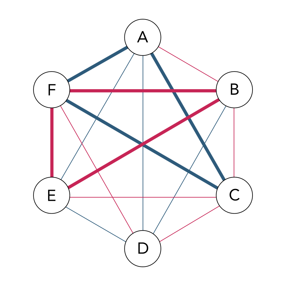
풀이. 임의의 정점에서 뻗어 나오는 간선의 개수는 5개이므로, 비둘기집의 원리에 따라 그중 적어도 3개는 같은 색을 가진다. 일반성을 잃지 않고, 간선 AB, AC, AD가 모두 빨간색이라고 하자. 만약 간선 BC, CD, DB 중 어느 하나가 빨간색이라면 세 변의 색이 모두 빨간색인 삼각형이 있다. 예를 들어 BC가 빨간색이라면 삼각형 ABC가 그러하다. 한편 BC, CD, DB가 모두 파란색이라면 삼각형 BCD는 세 변의 색이 모두 파란색이다. 따라서 세 변의 색이 모두 같은 삼각형이 적어도 하나 존재한다. ■

램지 정리

위 문제의 결론은 다음과 같이 표현할 수 있다. $G$가 정점수 6 이상인 완전 그래프일 때, $G$의 간선을 빨간색이나 파란색으로 칠하면 모든 간선이 빨간색인 정점수 3 이상의 부분 완전 그래프가 존재하거나, 모든 간선이 파란색인 정점수 3 이상의 부분 완전 그래프가 존재한다.

이 결론을 일반화하여, 다음 질문을 던질 수 있다. $r, b$가 임의의 자연수라고 하자. $G$가 정점수 $j$ 이상인 완전 그래프일 때, $G$의 간선을 빨간색이나 파란색으로 칠하면 모든 간선이 빨간색인 정점수 $r$ 이상의 부분 완전 그래프가 존재하거나, 모든 간선이 파란색인 정점수 $b$ 이상의 부분 완전 그래프가 존재함이 보장되는 자연수 $j$가 존재하는가?

램지 정리에 따르면 답은 그렇다이다. 구체적으로, 그러한 $j$ 중 가장 작은 수를 $R(r, b)$로 정의할 때, 다음이 성립한다.

램지 정리. 임의의 자연수 $r, b$에 대해 $R(r, b)$가 존재한다.

증명. $r + b$에 대한 귀납법으로 증명한다. 다음이 성립함을 보이면 충분한다.

\[R(r, b) \leq R(r-1, b) + R(r, b-1)\]

$R(r-1, b) = i, R(r, b-1) = j$라고 하자. $G$가 정점수 $i + j$인 완전 그래프라고 하고, $G$의 간선이 빨간색 또는 파란색으로 색칠되었다고 하자. 임의의 정점 $v \in G$에 대해, $v$와 빨간색 간선으로 연결된 정점들이 이루는 부분 완전 그래프를 $R$, 파란색 간선으로 연결된 정점들이 이루는 부분 완전 그래프를 $B$라고 하자. 다음이 성립한다.

\[|R| + |B| + 1 = i + j\]

따라서 다음 중 하나가 성립해야 한다.

1. $|R| \geq i$
2. $|B| \geq j$

1의 경우, $R(r-1, b) = i$이므로 $R$은 모든 간선이 빨간색인 정점수 $r-1$의 부분 완전 그래프를 가지거나, 모든 간선이 파란색인 정점수 $b$의 부분 완전 그래프를 가진다. 후자의 경우 $R(r, b)$의 조건이 충족되고, 전자의 경우 해당 그래프에 $v$를 추가한 그래프가 $R(r, b)$의 조건을 충족한다. 2의 경우도 마찬가지 논리가 성립한다. ■

서두의 문제는 $R(3, 3) \leq 6$임을 시사한다. 그리고 정점수가 5인 그래프 중에서는 문제의 조건을 만족하지 않는 그래프가 있음이 알려져 있기 때문에, $R(3, 3) = 6$이다. 또한 다음이 자명하다.

• $R(r, b) = R(b, r)$
• $R(r, 2) = r$

그러나 일반적인 값에 대해 램지 수를 정확히 계산하는 것은 매우 어려운 문제이다. 그래프의 정점 수에 따라 탐색해야 하는 경우의 수가 지수적 증가보다 빠르게 증가하기 때문이다. 현재 알려진 가장 빠른 램지 수 탐색 알고리즘의 시간 복잡도는 $O(c^{n^2})$이다. $R(5, 5)$의 값을 구하는 문제는 아직도 미해결 문제이며, 다만 43 이상 48 이하라는 사실이 알려져 있다. 이에 관해 다음 일화가 전해진다.

에르되시는 이런 이야기를 한 적이 있다. 우리보다 훨씬 진보한 외계 군단이 지구에 착륙해서는, $R(5, 5)$의 값을 계산해 내놓지 않는다면 지구를 산산조각낼 것이라 말했다고 상상해 보자. 에르되시가 주장하길, 이 경우에는 우리가 가진 모든 컴퓨터와 수학자를 모아들여서 계산을 시도해 봐야 한다. 그러나 만약 그들이 요구한 값이 $R(6, 6)$이라면, 에르되시 왈 이 경우에는 외계 군단을 무찌를 계획을 세우는 편이 낫다.¹

다수의 색에 대한 램지 정리

두 가지보다 많은 색을 사용하는 경우에도 램지 정리가 성립한다. 먼저 $R(n_1, n_2, \dots, n_k) = j$를, $k$가지 색을 사용하여 정점수가 $j$인 완전 그래프의 간선을 색칠했을 때 다음 중 적어도 하나가 언제나 존재하게 되는 가장 작은 $j$로 정의하자.

• 모든 간선이 1번째 색인 정점수 $n_1$의 부분 완전 그래프
• 모든 간선이 2번째 색인 정점수 $n_2$의 부분 완전 그래프
• …
• 모든 간선이 $k$번째 색인 정점수 $n_k$의 부분 완전 그래프

예를 들어 $R(3, 3, 3) = 17$임이 알려져 있다. 이는 정점수가 17 이상인 완전 그래프의 간선을 빨간색, 파란색, 또는 노란색으로 색칠하면 세 변의 색이 모두 빨간색이거나, 파란색이거나, 노란색인 삼각형이 언제나 존재한다는 의미이다.

다수의 색에 대한 램지 정리. 임의의 자연수 $n_1, \dots, n_k$에 대해 $R(n_1, \dots, n_k)$가 존재한다.

증명. $k$에 대한 귀납법으로 증명한다. 다음이 성립함을 보이면 충분하다.

\[R(n_1, \dots, n_k) \leq R(n_1, \dots, n_{k-2}, R(n_{k-1}, n_k))\]

부등식의 우변을 $j$라고 하자. $G$가 정점수 $j$인 완전 그래프라고 하고, $G$의 간선을 $k$개의 색을 사용하여 색칠하자. 잠시 $k - 1$번째 색과 $k$번째 색을 동일시하자. 그렇다면 $j$의 정의에 의해 다음 중 적어도 하나가 $G$에 존재한다.

• 모든 간선이 1번째 색인 정점수 $n_1$의 부분 완전 그래프
• 모든 간선이 2번째 색인 정점수 $n_2$의 부분 완전 그래프
• …
• 모든 간선이 $k-2$번째 색인 정점수 $n_{k-2}$의 부분 완전 그래프
• 모든 간선이 $k - 1$번째 색 = $k$번째 색인 정점수 $R(n_{k-1}, n_k)$의 부분 완전 그래프

마지막 경우를 제외하고는 $R(n_1, \dots, n_k)$의 조건을 만족하므로, 마지막 경우만 고려하면 된다. 마지막 경우가 보장하는 부분 완전 그래프를 $H$라고 하자. $R(n_{k-1}, n_k)$의 정의에 의해 $H$는 다음 중 적어도 하나를 가진다.

• 모든 간선이 $k-1$번째 색인 정점수 $n_{k-1}$의 부분 완전 그래프
• 모든 간선이 $k$번째 색인 정점수 $n_k$의 부분 완전 그래프

각 경우가 $R(n_1, \dots, n_k)$의 조건을 만족하므로, 모든 경우에 대해 $G$는 $R(n_1, \dots, n_k)$를 만족한다. ■

에르되시-라도 화살표

지금까지 우리는 간선의 색칠을 살펴 보았다. 간선은 두 정점 사이의 관계이다. 여기서 나아가, $n$개의 정점 사이의 관계를 색칠하는 상황을 떠올릴 수 있다.

논의의 편의를 위해 몇 가지 정의를 도입하자. 먼저 집합론적 자연수의 정의를 채택하여, $n = \lbrace0, 1, \dots, n-1\rbrace$로 정의한다. 또한 다음의 표기를 도입한다.

정의. $A$가 집합일 때, 다음과 같이 정의한다.

\[A^{(n)} = \{ S: S \subset A, |S| = n \}\]

즉, 자연수 $j$에 대해 $j^{(n)}$은 $_jC_n$의 각 경우를 원소로 가지는 집합이다. 예를 들어,

\[4^{(2)} = \bigg\{ \{ 0, 1\}, \{0, 2 \}, \{0, 3\}, \{1, 2 \}, \{1, 3\}, \{2, 3\} \bigg\}\]

주어진 집합을 $m$으로 분할한다는 것은, 집합의 각 원소를 $m$개의 범주 중 하나로 분류하는 것을 말한다. 예를 들어 $4^{(2)}$를 3개로 분류한 한 가지 결과는 다음과 같다.

\[\bigg\{ \big\{ \{0, 1\}, \{ 0, 2 \}, \{1, 2\} \big\}, \big\{ \{0, 3\}, \{2, 3 \} \big\}, \big\{ \{1, 3 \} \big\} \bigg\}\]

위 분할에서 $0, 1, 2$끼리 이루어진 집합은 모두 같은 범주에 속해 있다. 이것을 두고 $0, 1, 2$는 해당 분할에 대해 동질적_homogeneous이라고 한다.

다음의 표기를 정의한다. 이 표기를 에르되시-라도 화살표_{Erdős-Rado arrow}라고 부른다.

정의. $j^{(n)}$을 $m$으로 분할할 때 동질적인 $k$개의 원소가 언제나 존재할 경우 다음과 같이 표기한다.

\[j \rightarrow (k)^n_m\]

서두의 문제는 $6 \rightarrow (3)^2_2$임을 시사한다. $n = 2$인 이유는 간선이 두 정점 사이의 관계이기 때문이고, $m = 2$인 이유는 색이 두 가지이기 때문이다.

앞서 본 램지 정리에 의해 다음이 성립한다.

\[\forall k\; \exists j: j \to (k)^2_2\]

한편 다수의 색에 대한 램지 정리는 다음을 시사한다.

\[\forall k, m \; \exists j : j \to (k)^2_m\]

일반적으로 다음이 알려져 있다.

유한 에르되시-라도 정리. 임의의 자연수 $n, m, k$에 대해, 다음을 만족하는 자연수 $j$가 존재한다.

\[j \rightarrow (k)^n_m\]

무한 램지 정리

흥미롭게도 램지 정리는 $k$가 무한 기수_cardinal일 때에도 성립한다. 다음이 알려져 있다.

에르되시-라도 정리. 임의의 기수 $\lambda$와 자연수 $n, m$에 대해, 다음을 만족하는 기수 $\kappa$가 존재한다.

\[\kappa \rightarrow (\lambda)^n_m\]

특히 다음이 성립한다.

무한 램지 정리. \(\aleph_0 \rightarrow (\aleph_0)^n_m\)

즉 힐베르트 호텔의 투숙객들이 임의로 악수를 나눌 때, 서로 모두 악수를 나눈 사람들이 무한히 많거나, 서로 전혀 악수를 나누지 않은 사람들이 무한히 많다.

위 정리에 대한 증명은 필자 뇌피셜이기 때문에 오류가 있다면 알려주길 바란다.

증명. $n = m = 2$인 경우에 대해 증명한다. $G$가 크기가 $\aleph_0$인 완전 그래프라고 하자. $G$의 간선들을 빨간색 또는 파란색으로 색칠한다. $G$의 정점 $v, w$에 대해, $\overline{vw}$가 빨간색이면 $\overline{vw} \in R$, 파란색이면 $\overline{vw} \in B$와 같이 표현하자.

임의의 $G$의 정점 $v_0$에 대해, 다음과 같이 정의하자.

\[\begin{aligned} R_1 = \{ w \in G : \overline{v_0w} \in R \}\\ B_1 = \{ w \in G : \overline{v_0w} \in B \} \end{aligned}\]

$R_1 \cup B_1 \cup \lbrace v_0 \rbrace = G$이므로, $R_1$과 $B_1$ 중 적어도 하나는 무한집합이다. 만약 $R_1$이 무한집합이라면 $v_0 \in R$와 같이 표기하고, $B_1$이 무한집합이라면 $v_0 \in B$와 같이 표기하자.

$R_1$이 무한집합이라고 가정하자. 선택 공리로부터 $R_1$의 원소 $v_1$을 선택할 수 있다. 이제 다음과 같이 정의하자.

\[\begin{aligned} R_2 = \{ w \in R_1 : \overline{v_1w} \in R \}\\ B_2 = \{ w \in R_1 : \overline{v_1w} \in B \} \end{aligned}\]

$R_2 \cup B_2 \cup \lbrace v_1\rbrace = R_1$이므로, $R_2$와 $B_2$ 중 적어도 하나는 무한집합이다. 마찬가지로 $R_2$가 무한집합이라면 $v_1 \in R$, $B_2$가 무한집합이라면 $v_1 \in B$와 같이 표기하자.

$B_2$가 무한집합이라고 가정하자. $B_2$의 원소 $v_2$를 선택하여 다음과 같이 정의하자.

\[\begin{aligned} R_3 = \{ w \in B_2 : \overline{v_2w} \in R \}\\ B_3 = \{ w \in B_2 : \overline{v_2w} \in B \} \end{aligned}\]

이같은 식으로 반복함으로써 다음의 정점열을 얻는다.

\[V = \{ v_0, v_1, v_2, v_3, \dots \}\]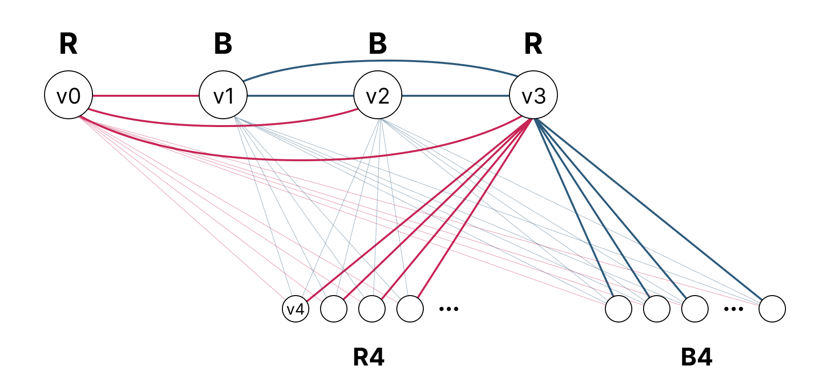

각 $v \in V$에 대해 $v \in R$ 또는 $v \in B$이다. $V$가 무한집합이므로, 다음 중 하나는 무한집합이다.

\[\begin{aligned} H = \{ v \in V : v \in R \} \\ K = \{ v \in V : v \in B \} \end{aligned}\]

만약 $H$가 무한집합이라면 $H$의 정점들이 이루는 완전 그래프는 간선의 색이 모두 빨간색이다. 한편 $K$가 무한집합이라면 $K$의 정점들이 이루는 완전 그래프는 간선의 색이 모두 파란색이다. 따라서 $\aleph_0 \rightarrow (\aleph_0)^2_2$이다. ■

따름정리. $A$가 $\mathbb{N}$의 무한 부분집합일 때, 어떤 $A$의 무한 부분집합 $B$가 존재하여 다음 중 하나가 성립한다.

• 임의의 $b \in B$에 대해, $c$가 $b$보다 큰 $B$의 원소라면 $b \mid c$이다.
• 임의의 $b, c \in B$에 대해, $b \nmid c, c \nmid b$이다.

증명. $k = A$로 잡고, $x < y$에 대해 $x \mid y$라면 $\lbrace x, y \rbrace$를 1번 범주로, 그렇지 않으면 2번 범주로 분류하는 분할을 고려한 뒤 $\aleph_0 \rightarrow (\aleph_0)^2_2$임을 사용한다. ■

무한에서 유한으로

흥미롭게도 콤팩트성 정리를 사용하면 무한 램지 정리로부터 유한 램지 정리를 증명할 수 있다. 즉, 다음이 성립한다.

보조정리. $\aleph_0 \rightarrow (\aleph_0)^n_m$라면, 임의의 자연수 $k$에 대해 $j \to (k)^n_m$을 만족하는 자연수 $j$가 존재한다.

증명. $n = 2$일 때를 증명한다. 간선이 $m$가지 색으로 색칠된 그래프는 다음과 같이 형식화할 수 있다. 먼저 언어 $\mathcal{L} = (V, f, 1, 2, \dots, m)$의 부호수_signature을 다음과 같이 정의한다.

• $V$는 단항 관계이다.
• $f$는 이변수 함수이다.
• $1, 2, \dots, m$은 상수이다.

$T$가 다음으로 이루어진 $\mathcal{L}$-이론이라고 하자.

• $\psi : \lnot V(1) \land \lnot V(2) \land \lnot V(m)$
• $\theta : \forall x, y \; (V(x) \land V(y) \land x \neq y) \rightarrow ( f(x, y) = 1 \lor f(x, y) = 2 \lor \cdots \lor f(x, y) = m )$
• $\phi_1 : \exists x_1, x_2 \; V(x_1) \land V(x_2) \land x_1 \neq x_2$
• $\phi_2 : \exists x_1, x_2, x_3 \; V(x_1) \land V(x_2) \land V(x_3) \land x_1 \neq x_2 \land x_2 \neq x_3 \neq x_1 \neq x_3$
• 각 $n \in \mathbb{N}$에 대해, $\phi_n$

$\psi$는 $1, 2, \dots, m$이 정점이 아니라 색을 표현한다는 의미이다. $\theta$는 임의의 두 정점 간 간선이 $1$부터 $m$ 중 하나의 색을 가짐을 의미한다. 그리고 $\phi_n$은 적어도 $n$개의 정점이 존재한다는 의미이다. 임의의 $n$에 대해 $\phi_n \in T$이므로, $T$의 모델은 무한 완전 그래프이다.

다음의 문장을 $\chi$라고 하자.

\[\exists x_1, x_2, \dots, x_k : f(x_1, x_2) = f(x_1, x_3) = \dots = f(x_{k-1}, x_k)\]

즉, $\chi$는 정점수 $k$인 동색의 부분 완전 그래프가 존재한다는 의미이다. 따라서 무한 램지 정리에 따라 다음이 성립한다.

\[T \vDash \psi\]

그리고 콤팩트성 정리에 따라 어떤 유한 부분이론 $T’ = \lbrace \psi, \chi, \phi_1, \dots, \phi_j \rbrace$가 존재하여 다음이 성립한다.

\[T' \vDash \psi\]

즉, 정점수 $j$ 이상인 모든 완전 그래프는 $\psi$를 만족한다. 다시 말해, $j \to (k)^2_m$이다. 임의의 $n$에 대해서 증명하려면 $R$을 $n$항 관계로 두면 된다. ■

¹ Joel H. Spencer (1994), Ten Lectures on the Probabilistic Method

Ramsey Numbers and the Infinite Ramsey Theorem

20 Feb 2025

This post was originally written in Korean, and has been machine translated into English. It may contain minor errors or unnatural expressions. Proofreading will be done in the near future.

Abstract. We examine the definition of Ramsey numbers and the Ramsey theorem that ensures Ramsey numbers are well-defined, extending this to infinite graphs. We also introduce an argument that derives the finite Ramsey theorem from the infinite Ramsey theorem using the compactness theorem.

Introduction

Problem. When the edges of a complete graph with 6 vertices are coloured red or blue, show that there exists a triangle whose three edges are all the same colour.

For instance, in the following diagram, triangles ACF and BEF satisfy the problem’s conditions.

Solution. The number of edges emanating from any vertex is 5, so by the pigeonhole principle, at least 3 of them have the same colour. Without loss of generality, suppose edges AB, AC, and AD are all red. If any one of edges BC, CD, or DB is red, then there exists a triangle with all three edges red. For example, if BC is red, then triangle ABC satisfies this condition. On the other hand, if BC, CD, and DB are all blue, then triangle BCD has all three edges blue. Therefore, there exists at least one triangle with all three edges the same colour. ■

Ramsey Theorem

The conclusion of the above problem can be expressed as follows: When $G$ is a complete graph with 6 or more vertices, if the edges of $G$ are coloured red or blue, then either there exists a complete subgraph with 3 or more vertices whose edges are all red, or there exists a complete subgraph with 3 or more vertices whose edges are all blue.

Generalising this conclusion, we can pose the following question: Let $r$ and $b$ be arbitrary natural numbers. Does there exist a natural number $j$ such that when $G$ is a complete graph with $j$ or more vertices and the edges of $G$ are coloured red or blue, it is guaranteed that either there exists a complete subgraph with $r$ or more vertices whose edges are all red, or there exists a complete subgraph with $b$ or more vertices whose edges are all blue?

According to the Ramsey theorem, the answer is yes. Specifically, when the smallest such $j$ is defined as $R(r, b)$, the following holds:

Ramsey Theorem. For any natural numbers $r$ and $b$, $R(r, b)$ exists.

Proof. We prove by induction on $r + b$. It suffices to show that the following holds:

\[R(r, b) \leq R(r-1, b) + R(r, b-1)\]

Let $R(r-1, b) = i$ and $R(r, b-1) = j$. Suppose $G$ is a complete graph with $i + j$ vertices, and the edges of $G$ are coloured red or blue. For any vertex $v \in G$, let $R$ be the complete subgraph formed by vertices connected to $v$ by red edges, and let $B$ be the complete subgraph formed by vertices connected by blue edges. The following holds:

\[|R| + |B| + 1 = i + j\]

Therefore, one of the following must hold:

1. $

   R

   \geq i$

2. $

   B

   \geq j$

In case 1, since $R(r-1, b) = i$, $R$ either has a complete subgraph with $r-1$ vertices whose edges are all red, or has a complete subgraph with $b$ vertices whose edges are all blue. In the latter case, the condition for $R(r, b)$ is satisfied, and in the former case, the graph obtained by adding $v$ to that subgraph satisfies the condition for $R(r, b)$. The same logic applies to case 2. ■

The problem at the beginning suggests that $R(3, 3) \leq 6$. Since it is known that there exist graphs with 5 vertices that do not satisfy the problem’s conditions, we have $R(3, 3) = 6$. The following are also trivial:

• $R(r, b) = R(b, r)$
• $R(r, 2) = r$

However, calculating Ramsey numbers exactly for general values is an extremely difficult problem. This is because the number of cases to be explored increases faster than exponentially with the number of vertices in the graph. The time complexity of the currently known fastest Ramsey number search algorithm is $O(c^{n^2})$. The problem of finding the value of $R(5, 5)$ remains unsolved, though it is known to be between 43 and 48 inclusive. The following anecdote is told regarding this:

Erdős once told this story. Imagine that a much more advanced alien force lands on Earth and says that unless we calculate the value of $R(5, 5)$, they will blow the Earth to pieces. Erdős claimed that in this case, we should gather all our computers and mathematicians to attempt the calculation. However, if they demanded the value of $R(6, 6)$, Erdős said it would be better to devise a plan to defeat the alien force.¹

Ramsey Theorem for Multiple Colours

The Ramsey theorem also holds when more than two colours are used. First, let us define $R(n_1, n_2, \ldots, n_k) = j$ as the smallest $j$ such that when the edges of a complete graph with $j$ vertices are coloured using $k$ colours, at least one of the following always exists:

• A complete subgraph with $n_1$ vertices whose edges are all the 1st colour
• A complete subgraph with $n_2$ vertices whose edges are all the 2nd colour
• …
• A complete subgraph with $n_k$ vertices whose edges are all the $k$th colour

For example, it is known that $R(3, 3, 3) = 17$. This means that when the edges of a complete graph with 17 or more vertices are coloured red, blue, or yellow, there always exists a triangle whose three edges are all red, all blue, or all yellow.

Ramsey Theorem for Multiple Colours. For any natural numbers $n_1, \ldots, n_k$, $R(n_1, \ldots, n_k)$ exists.

Proof. We prove by induction on $k$. It suffices to show that the following holds:

\[R(n_1, \ldots, n_k) \leq R(n_1, \ldots, n_{k-2}, R(n_{k-1}, n_k))\]

Let $j$ be the right-hand side of the inequality. Suppose $G$ is a complete graph with $j$ vertices, and colour the edges of $G$ using $k$ colours. Temporarily identify the $(k-1)$th colour with the $k$th colour. Then, by the definition of $j$, at least one of the following exists in $G$:

• A complete subgraph with $n_1$ vertices whose edges are all the 1st colour
• A complete subgraph with $n_2$ vertices whose edges are all the 2nd colour
• …
• A complete subgraph with $n_{k-2}$ vertices whose edges are all the $(k-2)$th colour
• A complete subgraph with $R(n_{k-1}, n_k)$ vertices whose edges are all the $(k-1)$th colour = $k$th colour

Except for the last case, the condition for $R(n_1, \ldots, n_k)$ is satisfied, so we need only consider the last case. Let $H$ be the complete subgraph guaranteed by the last case. By the definition of $R(n_{k-1}, n_k)$, $H$ has at least one of the following:

• A complete subgraph with $n_{k-1}$ vertices whose edges are all the $(k-1)$th colour
• A complete subgraph with $n_k$ vertices whose edges are all the $k$th colour

Since each case satisfies the condition for $R(n_1, \ldots, n_k)$, in all cases $G$ satisfies $R(n_1, \ldots, n_k)$. ■

Erdős-Rado Arrow

So far, we have examined the colouring of edges. Edges are relationships between two vertices. Going further, we can consider situations where relationships among $n$ vertices are coloured.

For convenience of discussion, let us introduce several definitions. First, we adopt the set-theoretic definition of natural numbers, defining $n = {0, 1, \ldots, n-1}$. We also introduce the following notation:

Definition. When $A$ is a set, we define:

\[A^{(n)} = \{ S: S \subset A, |S| = n \}\]

That is, for a natural number $j$, $j^{(n)}$ is a set whose elements are each case of $_jC_n$. For example,

\[4^{(2)} = \left\{ \{ 0, 1\}, \{0, 2 \}, \{0, 3\}, \{1, 2 \}, \{1, 3\}, \{2, 3\} \right\}\]

To partition a given set into $m$ parts means to classify each element of the set into one of $m$ categories. For example, one result of partitioning $4^{(2)}$ into 3 parts is:

\[\left\{ \left\{ \{0, 1\}, \{ 0, 2 \}, \{1, 2\} \right\}, \left\{ \{0, 3\}, \{2, 3 \} \right\}, \left\{ \{1, 3 \} \right\} \right\}\]

In the above partition, the sets formed by 0, 1, and 2 all belong to the same category. We say that 0, 1, and 2 are homogeneous with respect to this partition.

We define the following notation, called the Erdős-Rado arrow:

Definition. If there always exist $k$ homogeneous elements when $j^{(n)}$ is partitioned into $m$ parts, we write:

\[j \rightarrow (k)^n_m\]

The problem at the beginning suggests that $6 \rightarrow (3)^2_2$. The reason $n = 2$ is that edges are relationships between two vertices, and $m = 2$ because there are two colours.

By the Ramsey theorem we saw earlier, the following holds:

\[\forall k\; \exists j: j \to (k)^2_2\]

Meanwhile, the Ramsey theorem for multiple colours suggests:

\[\forall k, m \; \exists j : j \to (k)^2_m\]

In general, the following is known:

Finite Erdős-Rado Theorem. For any natural numbers $n$, $m$, and $k$, there exists a natural number $j$ such that:

\[j \rightarrow (k)^n_m\]

Infinite Ramsey Theorem

Interestingly, the Ramsey theorem also holds when $k$ is an infinite cardinal. The following is known:

Erdős-Rado Theorem. For any cardinal $\lambda$ and natural numbers $n$ and $m$, there exists a cardinal $\kappa$ such that:

\[\kappa \rightarrow (\lambda)^n_m\]

In particular, the following holds:

Infinite Ramsey Theorem. \(\aleph_0 \rightarrow (\aleph_0)^n_m\)

That is, when guests at Hilbert’s hotel arbitrarily shake hands, either there are infinitely many people who all shake hands with each other, or there are infinitely many people who never shake hands with each other.

The proof of the above theorem is the author’s own conjecture, so please let me know if there are any errors.

Proof. We prove for the case $n = m = 2$. Suppose $G$ is a complete graph of size $\aleph_0$. Colour the edges of $G$ red or blue. For vertices $v$ and $w$ of $G$, if $\overline{vw}$ is red, we write $\overline{vw} \in R$; if blue, we write $\overline{vw} \in B$.

For any vertex $v_0$ of $G$, define:

\[\begin{aligned} R_1 = \{ w \in G : \overline{v_0w} \in R \}\\ B_1 = \{ w \in G : \overline{v_0w} \in B \} \end{aligned}\]

Since $R_1 \cup B_1 \cup {v_0} = G$, at least one of $R_1$ and $B_1$ is an infinite set. If $R_1$ is infinite, we write $v_0 \in R$; if $B_1$ is infinite, we write $v_0 \in B$.

Suppose $R_1$ is infinite. By the axiom of choice, we can select an element $v_1$ of $R_1$. Now define:

\[\begin{aligned} R_2 = \{ w \in R_1 : \overline{v_1w} \in R \}\\ B_2 = \{ w \in R_1 : \overline{v_1w} \in B \} \end{aligned}\]

Since $R_2 \cup B_2 \cup {v_1} = R_1$, at least one of $R_2$ and $B_2$ is infinite. Similarly, if $R_2$ is infinite, we write $v_1 \in R$; if $B_2$ is infinite, we write $v_1 \in B$.

Suppose $B_2$ is infinite. Select an element $v_2$ of $B_2$ and define:

\[\begin{aligned} R_3 = \{ w \in B_2 : \overline{v_2w} \in R \}\\ B_3 = \{ w \in B_2 : \overline{v_2w} \in B \} \end{aligned}\]

By repeating in this manner, we obtain the following sequence of vertices:

\[V = \{ v_0, v_1, v_2, v_3, \ldots \}\]

For each $v \in V$, either $v \in R$ or $v \in B$. Since $V$ is infinite, one of the following is infinite:

\[\begin{aligned} H = \{ v \in V : v \in R \} \\ K = \{ v \in V : v \in B \} \end{aligned}\]

If $H$ is infinite, then the complete graph formed by the vertices of $H$ has all edges red. On the other hand, if $K$ is infinite, then the complete graph formed by the vertices of $K$ has all edges blue. Therefore, $\aleph_0 \rightarrow (\aleph_0)^2_2$. ■

Corollary. When $A$ is an infinite subset of $\mathbb{N}$, there exists an infinite subset $B$ of $A$ such that one of the following holds:

• For any $b \in B$, if $c$ is an element of $B$ greater than $b$, then $b \mid c$.
• For any $b, c \in B$, $b \nmid c$ and $c \nmid b$.

Proof. Take $k = A$, and consider a partition where for $x < y$, if $x \mid y$, then ${x, y}$ is classified into category 1; otherwise, into category 2. Then use the fact that $\aleph_0 \rightarrow (\aleph_0)^2_2$. ■

From Infinite to Finite

Interestingly, using the compactness theorem, one can prove the finite Ramsey theorem from the infinite Ramsey theorem. That is, the following holds:

Lemma. If $\aleph_0 \rightarrow (\aleph_0)^n_m$, then for any natural number $k$, there exists a natural number $j$ such that $j \to (k)^n_m$.

Proof. We prove for the case $n = 2$. A graph whose edges are coloured with $m$ colours can be formalised as follows. First, define the signature of language $\mathcal{L} = (V, f, 1, 2, \ldots, m)$ as:

• $V$ is a unary relation.
• $f$ is a binary function.
• $1, 2, \ldots, m$ are constants.

Let $T$ be an $\mathcal{L}$-theory consisting of:

• $\psi : \lnot V(1) \land \lnot V(2) \land \lnot V(m)$
• $\theta : \forall x, y \; (V(x) \land V(y) \land x \neq y) \rightarrow ( f(x, y) = 1 \lor f(x, y) = 2 \lor \cdots \lor f(x, y) = m )$
• $\phi_1 : \exists x_1, x_2 \; V(x_1) \land V(x_2) \land x_1 \neq x_2$
• $\phi_2 : \exists x_1, x_2, x_3 \; V(x_1) \land V(x_2) \land V(x_3) \land x_1 \neq x_2 \land x_2 \neq x_3 \land x_1 \neq x_3$
• For each $n \in \mathbb{N}$, $\phi_n$

$\psi$ means that $1, 2, \ldots, m$ represent colours, not vertices. $\theta$ means that any edge between two vertices has one of the colours from $1$ to $m$. And $\phi_n$ means that at least $n$ vertices exist. Since $\phi_n \in T$ for any $n$, models of $T$ are infinite complete graphs.

Let the following sentence be $\chi$:

\[\exists x_1, x_2, \ldots, x_k : f(x_1, x_2) = f(x_1, x_3) = \ldots = f(x_{k-1}, x_k)\]

That is, $\chi$ means that there exists a monochromatic complete subgraph with $k$ vertices. Therefore, according to the infinite Ramsey theorem, the following holds:

\[T \vDash \chi\]

And by the compactness theorem, there exists some finite sub-theory $T’ = {\psi, \theta, \phi_1, \ldots, \phi_j}$ such that:

\[T' \vDash \chi\]

That is, every complete graph with $j$ or more vertices satisfies $\chi$. In other words, $j \to (k)^2_m$. To prove for arbitrary $n$, one can take $R$ as an $n$-ary relation. ■

¹ Joel H. Spencer (1994), Ten Lectures on the Probabilistic Method

어드조인트, 정규 변환, 그리고 스펙트럼 정리

13 Feb 2025

이 글에서 모든 벡터 공간은 내적 공간이라고 가정한다. 또한, 모든 변환은 선형 변환이다.

1. 선형 변환의 어드조인트

정의. $(V, \langle \cdot \rangle_V), (W, \langle \cdot \rangle_W)$가 내적 벡터 공간이라고 하자. $T: V \to W$에 대해, $T$의 어드조인트_adjoint $T^\ast: W \to V$는 다음 조건을 만족하는 선형 변환이다.

\[\forall v \in V, w \in W : \quad \langle w, Tv \rangle_W = \langle T^\ast w, v \rangle_V\]

범주론의 어드조인트 정의를 떠올려 보면 식의 형태가 비슷하다.

이 정의를 정당화하려면 모든 $T$에 대해 어드조인트가 유일하게 존재함을 보여야 한다. 이는 리스 표현 정리_{Riesz representation theorem}로부터 얻어진다.

리스 표현 정리. $V$가 내적 공간이라고 하자. $\phi \in V^\ast$에 대해, 다음을 만족하는 벡터 $v$가 유일하게 존재한다.

\[\forall u \in V : \quad \phi(u) = \langle u, v \rangle\]

$V$가 유한 차원일 경우, 위 정리는 $V$의 직교 기저를 잡음으로써 쉽게 보여진다. $V$가 일반적인 힐베르트 공간일 경우에는 증명이 더 까다롭기 때문에 생략한다.

리스 표현 정리로부터 어드조인트의 정의를 다음과 같이 정당화할 수 있다. $w \in W$가 주어졌을 때, 사상 $v \mapsto \langle w, Tv \rangle$는 $V^\ast$의 원소이다. 따라서 어떤 $u_w \in V$가 존재하여

\[\forall v \in V : \langle w, Tv \rangle = \langle u_w, v \rangle\]

이다. 이때 사상 $w \mapsto u_w$는 선형임을 쉽게 보일 수 있다. 이 선형 사상이 우리가 구하고자 하는 어드조인트이다.

정의. $T^\ast = T$인 선형 사상 $T : V \to V$를 자기 어드조인트_self-adjoint라고 한다.

$T : V \to W$의 행렬 표현이 $M$일 때, 동일한 기저에서 $T^\ast$의 행렬 표현은 $M$의 켤레 전치, 즉 $M^\dagger$임을 — 다소 번거롭긴 하지만 — 어렵지 않게 보일 수 있다. 따라서 자기 어드조인트 변환의 행렬은 에르미트_Hermitian 행렬이다.

복소 자기 어드조인트 판별볍. $V$가 복소 벡터 공간일 때, $T: V \to V$가 자기 어드조인트 변환일 필요충분조건은 임의의 $v \in V$에 대해 $\langle Tv, v \rangle \in \mathbb{R}$인 것이다.

증명. 필요조건은 자명하므로 충분조건임을 보인다. 먼저 다음 보조정리를 증명한다.

보조정리. $V$가 복소 벡터 공간이라고 하자. $T : V \to V$에 대해, $T = 0$일 필요충분조건은 임의의 $v \in V$에 대해 $\langle Tv, v \rangle = 0$인 것이다.

보조정리의 증명. 필요조건은 자명하므로 충분조건임을 보인다. 임의의 $u, v \in V$에 대해,

\[\langle T(u + v) , u + v \rangle = \langle Tu, v \rangle + \langle Tv, u \rangle = 0\]

이고,

\[\begin{aligned} \langle T(u + iv), u + iv \rangle &= \langle T(u), iv \rangle + \langle T(iv), u \rangle \\ &= -i \langle Tu, v \rangle + i \langle Tv, u \rangle = 0 \end{aligned}\]

이다. 두 식을 연립하면 $\langle Tu, v \rangle = 0$을 얻는다. 이로부터 $T = 0$임을 보이기는 쉽다. □

이제 본 정리를 보인다. $\langle Tv, v \rangle \in \mathbb{R}$이므로, $\langle Tv, v \rangle = \langle v, Tv \rangle$이다. 또한 어드조인트의 정의에 의해 $\langle Tv, v \rangle = \langle v, T^\ast v \rangle$이다. 따라서 $\langle v, (T - T^\ast)v \rangle = 0$이다. 보조정리로부터 $T = T^\ast$가 따라 나온다. ■

자명한 자기 어드조인트 판별법. $V$가 실수 또는 복소 벡터 공간이라고 하자. 자기 어드조인트 변환 $T: V \to V$에 대해, $T = 0$일 필요충분조건은 임의의 $v \in V$에 대해 $\langle Tv, v \rangle = 0$인 것이다.

증명. 복소 벡터 공간인 경우에는 위의 보조정리로부터 따라 나온다. 따라서 $V$가 실수 벡터 공간인 경우에만 증명한다. 필요조건은 자명하므로 충분조건임을 보인다. 임의의 $u, v \in V$에 대해,

\[\begin{aligned} \langle T(u + v), u + v \rangle &= \langle Tu, v \rangle + \langle Tv, u \rangle &&(\because \langle Tv, v \rangle = 0) \\ &= \langle Tu, v \rangle + \langle u, Tv \rangle &&(\because \mathrm{im} \langle \cdot \rangle \subset \mathbb{R}) \\ &= 2\langle Tu, v \rangle &&(\because T^\ast = T) \end{aligned}\]

즉 임의의 $u, v \in V$에 대해 $\langle Tu, v \rangle = 0$이므로 $T = 0$이다. ■

2. 정규 선형 변환

정의. $T : V \to V$에 대해 $TT^\ast = T^\ast T$일 때, $T$를 정규_normal라고 한다.

모든 자기 어드조인트 변환은 정규 변환이지만 그 역은 성립하지 않는다.

정규 판별법. $V$가 실수 또는 복소 벡터 공간이라고 하자. $T: V \to V$가 정규일 필요충분조건은 임의의 $v$에 대해 $\lVert Tv \rVert = \lVert T^\ast v \rVert$인 것이다.

증명. “자명한 자기 어드조인트 판별법”으로부터 따라 나온다. ■

정규 고유벡터의 켤레성. $V$가 실수 또는 복소 벡터 공간이고, $T : V \to V$가 정규라고 하자. $v$가 고윳값 $\lambda$를 가지는 $T$의 고유벡터일 때, $v$는 고윳값 $\bar{\lambda}$를 가지는 $T^\ast$의 고유벡터이다.

증명. $T$가 정규일 때, $T - \lambda I$ 또한 정규임을 쉽게 보일 수 있다. 따라서,

\[\lVert (T - \lambda I) v \rVert = \lVert (T - \lambda I)^\ast v \rVert = \lVert (T^\ast - \bar{\lambda} I) v \rVert = 0. \quad \blacksquare\]

‘정규’라는 이름의 유래는 다음 정리에 있다.

정규 고유벡터의 정규성. $T: V \to V$가 정규라고 하자. $u, v \in V$가 서로 다른 고윳값을 가지는 $T$의 고유벡터라면 $u$와 $v$는 직교한다.

증명. $u, v$의 고윳값이 $\alpha, \beta$라고 하자.

\[\begin{aligned} (\alpha - \beta)\langle u, v \rangle &= \langle \alpha u, v \rangle - \langle u, \bar{\beta}v \rangle \\ &= \langle Tu, v \rangle - \langle u, T^\ast v \rangle = 0. \end{aligned}\]

$\alpha - \beta \neq 0$이므로 $\langle u, v \rangle = 0$이다. ■

3. 스펙트럼 정리_{Spectral theorems}

‘스펙트럼’이라는 이름은, 스펙트럼 정리가 양자역학에서 원자의 스펙트럼을 설명할 때 쓰였던 것에서 유래했다는 설이 흔히 전해지지만, 이것은 사실이 아니다. 스펙트럼 정리를 사용해서 원자의 스펙트럼을 설명하기 이전에 이미 힐베르트가 ‘스펙트럼’이라는 표현을 쓴 바 있기 때문이다. 정확한 유래는 알려져 있지 않은데, 고유벡터들이 힐베르트 공간의 특성을 나타낸다는 점에서 빛의 스펙트럼과 유사하다는 이미지 때문이 아니었을까 추측해 봄직하다.

복소 스펙트럼 정리. $V$가 복소 벡터 공간이라고 하자. $T: V \to V$가 정규일 필요충분조건은, $T$의 고유벡터들이 $V$의 직교 기저를 이루는 것이다.

증명. TODO ■

실수 스펙트럼 정리. $V$가 실수 벡터 공간이라고 하자. $T: V \to V$가 자기 어드조인트일 필요충분조건은, $T$의 고유벡터들이 $V$의 직교 기저를 이루는 것이다.

증명. TODO ■

Adjoints, Normal Transformations, and the Spectral Theorem

13 Feb 2025

This post was originally written in Korean, and has been machine translated into English. It may contain minor errors or unnatural expressions. Proofreading will be done in the near future.

In this article, we assume that all vector spaces are inner product spaces. Furthermore, all transformations are linear transformations.

1. Adjoints of Linear Transformations

Definition. Let $(V, \langle \cdot \rangle_V), (W, \langle \cdot \rangle_W)$ be inner product vector spaces. For $T: V \to W$, the adjoint $T^\ast: W \to V$ of $T$ is the linear transformation satisfying the following condition:

\[\forall v \in V, w \in W : \quad \langle w, Tv \rangle_W = \langle T^\ast w, v \rangle_V\]

If one recalls the definition of adjoints in category theory, the form of this equation is similar.

To justify this definition, we must show that the adjoint exists uniquely for every $T$. This follows from the Riesz representation theorem.

Riesz Representation Theorem. Let $V$ be an inner product space. For $\phi \in V^\ast$, there exists a unique vector $v$ satisfying:

\[\forall u \in V : \quad \phi(u) = \langle u, v \rangle\]

When $V$ is finite-dimensional, the above theorem is easily shown by choosing an orthogonal basis for $V$. When $V$ is a general Hilbert space, the proof is more involved and shall be omitted.

From the Riesz representation theorem, we can justify the definition of the adjoint as follows. Given $w \in W$, the mapping $v \mapsto \langle w, Tv \rangle$ is an element of $V^\ast$. Therefore, there exists some $u_w \in V$ such that

\[\forall v \in V : \langle w, Tv \rangle = \langle u_w, v \rangle\]

At this point, one can easily show that the mapping $w \mapsto u_w$ is linear. This linear mapping is the adjoint we seek.

Definition. A linear mapping $T : V \to V$ satisfying $T^\ast = T$ is called self-adjoint.

When the matrix representation of $T : V \to W$ is $M$, the matrix representation of $T^\ast$ in the same basis is the conjugate transpose of $M$, namely $M^\dagger$ — this can be shown, albeit somewhat tediously, without much difficulty. Therefore, the matrix of a self-adjoint transformation is a Hermitian matrix.

Complex Self-Adjoint Criterion. When $V$ is a complex vector space, $T: V \to V$ is self-adjoint if and only if $\langle Tv, v \rangle \in \mathbb{R}$ for any $v \in V$.

Proof. The necessary condition is trivial, so we prove the sufficient condition. First, we establish the following lemma.

Lemma. Let $V$ be a complex vector space. For $T : V \to V$, $T = 0$ if and only if $\langle Tv, v \rangle = 0$ for any $v \in V$.

Proof of the lemma. The necessary condition is trivial, so we prove the sufficient condition. For any $u, v \in V$,

\[\langle T(u + v) , u + v \rangle = \langle Tu, v \rangle + \langle Tv, u \rangle = 0\]

and

\[\begin{aligned} \langle T(u + iv), u + iv \rangle &= \langle T(u), iv \rangle + \langle T(iv), u \rangle \\ &= -i \langle Tu, v \rangle + i \langle Tv, u \rangle = 0 \end{aligned}\]

Solving these two equations simultaneously yields $\langle Tu, v \rangle = 0$. From this, it is easy to show that $T = 0$. □

We now prove the main theorem. Since $\langle Tv, v \rangle \in \mathbb{R}$, we have $\langle Tv, v \rangle = \langle v, Tv \rangle$. Also, by the definition of the adjoint, $\langle Tv, v \rangle = \langle v, T^\ast v \rangle$. Therefore, $\langle v, (T - T^\ast)v \rangle = 0$. From the lemma, it follows that $T = T^\ast$. ■

Trivial Self-Adjoint Criterion. Let $V$ be a real or complex vector space. For a self-adjoint transformation $T: V \to V$, $T = 0$ if and only if $\langle Tv, v \rangle = 0$ for any $v \in V$.

Proof. For complex vector spaces, this follows from the lemma above. Therefore, we prove only the case when $V$ is a real vector space. The necessary condition is trivial, so we prove the sufficient condition. For any $u, v \in V$,

\[\begin{aligned} \langle T(u + v), u + v \rangle &= \langle Tu, v \rangle + \langle Tv, u \rangle &&(\because \langle Tv, v \rangle = 0) \\ &= \langle Tu, v \rangle + \langle u, Tv \rangle &&(\because \mathrm{im} \langle \cdot \rangle \subset \mathbb{R}) \\ &= 2\langle Tu, v \rangle &&(\because T^\ast = T) \end{aligned}\]

That is, $\langle Tu, v \rangle = 0$ for any $u, v \in V$, so $T = 0$. ■

2. Normal Linear Transformations

Definition. For $T : V \to V$, when $TT^\ast = T^\ast T$, we call $T$ normal.

Every self-adjoint transformation is normal, but the converse does not hold.

Normal Criterion. Let $V$ be a real or complex vector space. $T: V \to V$ is normal if and only if $\lVert Tv \rVert = \lVert T^\ast v \rVert$ for any $v$.

Proof. This follows from the “Trivial Self-Adjoint Criterion”. ■

Conjugacy of Normal Eigenvectors. Let $V$ be a real or complex vector space, and let $T : V \to V$ be normal. When $v$ is an eigenvector of $T$ with eigenvalue $\lambda$, then $v$ is an eigenvector of $T^\ast$ with eigenvalue $\bar{\lambda}$.

Proof. When $T$ is normal, $T - \lambda I$ is also easily shown to be normal. Therefore,

\[\lVert (T - \lambda I) v \rVert = \lVert (T - \lambda I)^\ast v \rVert = \lVert (T^\ast - \bar{\lambda} I) v \rVert = 0. \quad \blacksquare\]

The origin of the name ‘normal’ lies in the following theorem.

Normality of Normal Eigenvectors. Let $T: V \to V$ be normal. If $u, v \in V$ are eigenvectors of $T$ with distinct eigenvalues, then $u$ and $v$ are orthogonal.

Proof. Let the eigenvalues of $u, v$ be $\alpha, \beta$ respectively.

\[\begin{aligned} (\alpha - \beta)\langle u, v \rangle &= \langle \alpha u, v \rangle - \langle u, \bar{\beta}v \rangle \\ &= \langle Tu, v \rangle - \langle u, T^\ast v \rangle = 0. \end{aligned}\]

Since $\alpha - \beta \neq 0$, we have $\langle u, v \rangle = 0$. ■

3. Spectral Theorems

while it is commonly claimed that the name ‘spectral’ derives from the spectral theorem being used to explain atomic spectra in quantum mechanics, this is not factual. Hilbert had already used the term ‘spectrum’ before the spectral theorem was employed to explain atomic spectra. The precise origin is unknown, but one might conjecture that it arose from the imagery that eigenvectors characterise the properties of Hilbert spaces, similar to how light spectra characterise light.

Complex Spectral Theorem. Let $V$ be a complex vector space. $T: V \to V$ is normal if and only if the eigenvectors of $T$ form an orthogonal basis for $V$.

Proof. TODO ■

Real Spectral Theorem. Let $V$ be a real vector space. $T: V \to V$ is self-adjoint if and only if the eigenvectors of $T$ form an orthogonal basis for $V$.

Proof. TODO ■

어드조인트에 대한 세 가지 접근

13 Feb 2025

본문의 내용은 Tom Leinster, Basic Category Theory에 기반한다.

$\mathcal{A}, \mathcal{B}$가 범주_category이고, $F: \mathcal{A} \to \mathcal{B}, G: \mathcal{B} \to \mathcal{A}$가 함자_functor라고 하자.

1. 자연성 공리_{naturality axiom}를 이용한 어드조인트의 정의

$F \dashv G$라는 것은 임의의 $A \in \mathcal{A}, B \in \mathcal{B}$에 대해 일대일대응 $\Psi_{A, B} : \mathrm{Hom}_\mathcal{A}(A, G(B)) \to \mathrm{Hom}_\mathcal{B}(F(A), B)$가 존재하여, 임의의 $p: A’ \to A, q: B \to B’$에 대해 다음 가환 도식_{commutative diagram}을 만족한다는 것이다.

편의를 위해 $f: A \to G(B)$에 대해 $\Psi_{A, B}(f) = \bar{f}$, 그리고 $g: F(A) \to B$에 대해 $\Psi_{A, B}^{-1}(g) = \bar{g}$와 같이 표기한다. 이에 따라 위의 가환 도식을 다음과 같이 표현할 수 있다.

\[\begin{gather} \overline{A \xrightarrow{f} G(B) \xrightarrow{G(q)} G(B') } = F(A) \xrightarrow{\bar{f}} B \xrightarrow{q} B' \\ \overline{F(A') \xrightarrow{F(p)} F(A) \xrightarrow{g} B} = A' \xrightarrow{p} A \xrightarrow{\bar{g}} G(B) \\\\ \mathrm{i.e.}\\\\ \overline{G(q) \circ f} = q \circ \bar{f}\\ \overline{g \circ F(p)} = \bar{g} \circ p \end{gather}\]

위 두 조건을 자연성 공리라고 부른다. 자연성 공리로부터 다음을 증명할 수 있다.

정리 1. $\eta_A := \overline{1_{F(A)}} : A \to GF(A)$와 같이 정의된 변환 $\eta: 1_{\mathcal{A}} \to GF$는 자연적 변환_{natural transformation}이다. 그리고 $\epsilon_B := \overline{1_{G(B)}} : FG(B) \to B$와 같이 정의된 변환 $\epsilon: FG \to 1_{\mathcal{B}}$ 또한 자연적 변환이다. $\eta$를 단원_unit이라고 부르고, $\epsilon$을 쌍단원_counit이라고 부른다.

증명. 다음 가환 도식으로부터 얻어진다.

정리 2. $f: A \to G(B), g: F(A) \to B$에 대해 다음이 성립한다.

\[\begin{gather} \bar{f} = \epsilon_B \circ F(f) \\ \bar{g} = G(g) \circ \eta_A \end{gather}\]

증명. 다음 가환 도식으로부터 얻어진다.

2. 단원과 쌍단원을 이용한 어드조인트의 정의

$F \dashv G$라는 것은 어떤 자연적 변환 $\eta: 1_{\mathcal{A}} \to GF, \epsilon: FG \to 1_{\mathcal{B}}$가 존재하여, 임의의 $A \in \mathcal{A}, B \in \mathcal{B}$에 대해 다음 가환 도식을 언제나 만족한다는 것이다.

위 두 조건을 삼각 항등식_{triangle identity}이라고 부른다.

3. 초기 대상_{initial object}을 이용한 어드조인트의 정의

정의. $P: \mathcal{A} \to \mathcal{C}$, $Q: \mathcal{B} \to \mathcal{C}$가 함자일 때, 콤마 범주_{comma category} $(P \Rightarrow Q)$를 다음과 같이 정의한다.

• 대상: $\mathcal{C}$의 사상 $h: P(A) \to Q(B)$에 대해, 삼중쌍_triplet $(A, h, B)$
• 사상: 다음의 가환 도식이 성립할 때, $(f, g): (A, h, B) \to (A’, h’, B’)$

$F \dashv G$라는 것은 어떤 자연적 변환 $\eta: 1_{\mathcal{A}} \to GF$가 존재하여, 각 $A \in \mathcal{A}$에 대해 $A$를 홑원소 범주 $\mathbf{1}$에서 $\mathcal{A}$로 가는 함자 $A: 1 \mapsto A$로 간주했을 때 $\eta_A : A \to GF(A)$가 콤마 범주 $(A \Rightarrow G)$의 초기 대상이라는 것이다.

4. 동치 증명

1, 2, 3의 정의는 모두 동치이다. 구체적으로 다음의 정리가 성립한다.

정리 3. $\mathcal{A}, \mathcal{B}$가 범주이고 $F: \mathcal{A} \to \mathcal{B}, G: \mathcal{B} \to \mathcal{A}$가 함자라고 하자. 1, 2, 3은 서로 일대일 대응된다.

1. 자연성 공리를 만족하는 일대일대응 $\Psi$
2. 삼각 항등식을 만족하는 자연적 변환의 쌍 $(\eta: 1_{\mathcal{A}} \to GF, \epsilon: FG \to 1_{\mathcal{B}})$
3. 각 $A \in \mathcal{A}$에 대해 $\eta_A : A \to GF(A)$가 $(A \Rightarrow G)$의 초기 대상이 되도록 하는 자연적 변환 $\eta: 1_{\mathcal{A}} \to GF$

증명. 1과 2가 일대일 대응됨을 보이고, 2와 3이 일대일 대응됨을 보인다.

1과 2는 일대일 대응된다.

$\Psi$가 주어졌을 때, $\eta$와 $\epsilon$을 각각 단원과 쌍단원으로 정의한다. 이때, $\eta$와 $\epsilon$이 삼각 항등식을 만족함은 정리 2로부터 쉽게 따라 나온다.

역으로 삼각 항등식을 만족하는 자연적 변환의 쌍 $(\eta, \epsilon)$이 주어졌다고 하자. 이로부터 다음과 같이 $\Psi$를 정의한다. $f: A \to G(B), g: F(A) \to B$에 대해,

\[\begin{gather} \Psi_{A, B}(f) = \bar{f} = \epsilon_B \circ F(f) \\ \Psi_{A, B}^{-1} = \bar{g} = G(g) \circ \eta_A \end{gather}\]

먼저 $\Psi_{A, B}^{-1}$이 실제로 $\Psi_{A, B}$의 역사상임을, 즉 $\bar{\bar{g}} = g, \bar{\bar{f}} = f$임을 보인다. 전자는 다음 가환 도식으로부터 얻어진다. 후자는 도식에서 $F, G$를 각각 $G, F$로 바꾼 뒤 적절히 쌍대_dual을 취하면 된다.

이제 $\Psi$가 자연성 공리를 만족함을 보인다. 한쪽 공리만 보이도록 한다. $f: A \to G(B), q: B \to B’$에 대해 $\overline{G(q) \circ f} = q \circ \bar{f}$임을 보인다. 먼저,

\[\overline{G(q) \circ f} = \epsilon_{B'} \circ FG(q) \circ F(f)\]

이고,

\[q \circ \bar{f} = q \circ \epsilon_B \circ F(f)\]

이므로, $\epsilon_{B’} \circ FG(q) = q \circ \epsilon_B$임을 보이면 충분하다. 이것은 자연적 변환의 정의에 다름 아니다. 따라서 $\Psi$는 자연성 공리를 만족한다.

2와 3은 일대일 대응된다.

삼각 항등식을 만족하는 자연적 변환의 쌍 $(\eta, \epsilon)$이 주어졌을 때, 각 $A \in \mathcal{A}$에 대해 $\eta_A : A \to GF(A)$가 $(A \Rightarrow G)$의 초기 대상임을 보이자.

역으로 $\eta$가 각 $A \in \mathcal{A}$에 대해 $\eta_A : A \to GF(A)$가 $(A \Rightarrow G)$의 초기 대상이 되도록 하는 자연적 변환일 때, 어떤 $\epsilon: FG \to 1_{\mathcal{B}}$가 유일하게 존재하여 $(\eta, \epsilon)$이 삼각 항등식을 만족함을 보이자.

Three Approaches to Adjoints

13 Feb 2025

This post was originally written in Korean, and has been machine translated into English. It may contain minor errors or unnatural expressions. Proofreading will be done in the near future.

The content of this text is based on Tom Leinster, Basic Category Theory.

Let $\mathcal{A}, \mathcal{B}$ be categories and $F: \mathcal{A} \to \mathcal{B}, G: \mathcal{B} \to \mathcal{A}$ be functors.

1. Definition of Adjoint Using the Naturality Axiom

$F \dashv G$ means that for any $A \in \mathcal{A}, B \in \mathcal{B}$, there exists a bijection $\Psi_{A, B} : \mathrm{Hom}_\mathcal{A}(A, G(B)) \to \mathrm{Hom}_\mathcal{B}(F(A), B)$ such that for any $p: A’ \to A, q: B \to B’$, the following commutative diagram is satisfied.

For convenience, we denote $\Psi_{A, B}(f) = \bar{f}$ for $f: A \to G(B)$, and $\Psi_{A, B}^{-1}(g) = \bar{g}$ for $g: F(A) \to B$. Accordingly, the above commutative diagram can be expressed as follows:

\[\begin{gather} \overline{A \xrightarrow{f} G(B) \xrightarrow{G(q)} G(B') } = F(A) \xrightarrow{\bar{f}} B \xrightarrow{q} B' \\ \overline{F(A') \xrightarrow{F(p)} F(A) \xrightarrow{g} B} = A' \xrightarrow{p} A \xrightarrow{\bar{g}} G(B) \\\\ \mathrm{i.e.}\\\\ \overline{G(q) \circ f} = q \circ \bar{f}\\ \overline{g \circ F(p)} = \bar{g} \circ p \end{gather}\]

The above two conditions are called the naturality axioms. From the naturality axioms, we can prove the following:

Theorem 1. The transformation $\eta: 1_{\mathcal{A}} \to GF$ defined by $\eta_A := \overline{1_{F(A)}} : A \to GF(A)$ is a natural transformation. Moreover, the transformation $\epsilon: FG \to 1_{\mathcal{B}}$ defined by $\epsilon_B := \overline{1_{G(B)}} : FG(B) \to B$ is also a natural transformation. We call $\eta$ the unit and $\epsilon$ the counit.

Proof. This follows from the following commutative diagram.

Theorem 2. For $f: A \to G(B), g: F(A) \to B$, the following holds:

\[\begin{gather} \bar{f} = \epsilon_B \circ F(f) \\ \bar{g} = G(g) \circ \eta_A \end{gather}\]

Proof. This follows from the following commutative diagram.

2. Definition of Adjoint Using Unit and Counit

$F \dashv G$ means that there exist natural transformations $\eta: 1_{\mathcal{A}} \to GF$ and $\epsilon: FG \to 1_{\mathcal{B}}$ such that for any $A \in \mathcal{A}, B \in \mathcal{B}$, the following commutative diagrams are always satisfied:

The above two conditions are called the triangle identities.

3. Definition of Adjoint Using Initial Objects

Definition. When $P: \mathcal{A} \to \mathcal{C}$ and $Q: \mathcal{B} \to \mathcal{C}$ are functors, we define the comma category $(P \Rightarrow Q)$ as follows:

• Objects: For a morphism $h: P(A) \to Q(B)$ in $\mathcal{C}$, the triplet $(A, h, B)$
• Morphisms: When the following commutative diagram holds, $(f, g): (A, h, B) \to (A’, h’, B’)$

$F \dashv G$ means that there exists a natural transformation $\eta: 1_{\mathcal{A}} \to GF$ such that for each $A \in \mathcal{A}$, when we regard $A$ as a functor $A: 1 \mapsto A$ from the singleton category $\mathbf{1}$ to $\mathcal{A}$, $\eta_A : A \to GF(A)$ is an initial object in the comma category $(A \Rightarrow G)$.

4. Proof of Equivalence

The definitions 1, 2, and 3 are all equivalent. Specifically, the following theorem holds:

Theorem 3. Let $\mathcal{A}, \mathcal{B}$ be categories and $F: \mathcal{A} \to \mathcal{B}, G: \mathcal{B} \to \mathcal{A}$ be functors. Then 1, 2, and 3 are in one-to-one correspondence.

1. A bijection $\Psi$ satisfying the naturality axioms
2. A pair of natural transformations $(\eta: 1_{\mathcal{A}} \to GF, \epsilon: FG \to 1_{\mathcal{B}})$ satisfying the triangle identities
3. A natural transformation $\eta: 1_{\mathcal{A}} \to GF$ such that for each $A \in \mathcal{A}$, $\eta_A : A \to GF(A)$ is an initial object in $(A \Rightarrow G)$

Proof. We show that 1 and 2 are in one-to-one correspondence, and that 2 and 3 are in one-to-one correspondence.

1 and 2 are in one-to-one correspondence.

Given $\Psi$, we define $\eta$ and $\epsilon$ as the unit and counit respectively. That $\eta$ and $\epsilon$ satisfy the triangle identities follows easily from Theorem 2.

Conversely, suppose we are given a pair of natural transformations $(\eta, \epsilon)$ satisfying the triangle identities. From this, we define $\Psi$ as follows. For $f: A \to G(B), g: F(A) \to B$:

\[\begin{gather} \Psi_{A, B}(f) = \bar{f} = \epsilon_B \circ F(f) \\ \Psi_{A, B}^{-1} = \bar{g} = G(g) \circ \eta_A \end{gather}\]

First, we show that $\Psi_{A, B}^{-1}$ is indeed the inverse of $\Psi_{A, B}$, i.e., that $\bar{\bar{g}} = g, \bar{\bar{f}} = f$. The former follows from the following commutative diagram. The latter can be obtained by replacing $F, G$ with $G, F$ respectively in the diagram and then taking the appropriate dual.

Now we show that $\Psi$ satisfies the naturality axioms. We shall prove only one axiom. For $f: A \to G(B), q: B \to B’$, we show that $\overline{G(q) \circ f} = q \circ \bar{f}$. First,

\[\overline{G(q) \circ f} = \epsilon_{B'} \circ FG(q) \circ F(f)\]

and

\[q \circ \bar{f} = q \circ \epsilon_B \circ F(f)\]

Therefore, it suffices to show that $\epsilon_{B’} \circ FG(q) = q \circ \epsilon_B$. This is nothing other than the definition of a natural transformation. Hence $\Psi$ satisfies the naturality axioms.

2 and 3 are in one-to-one correspondence.

Given a pair of natural transformations $(\eta, \epsilon)$ satisfying the triangle identities, let us show that for each $A \in \mathcal{A}$, $\eta_A : A \to GF(A)$ is an initial object in $(A \Rightarrow G)$.

Conversely, when $\eta$ is a natural transformation such that for each $A \in \mathcal{A}$, $\eta_A : A \to GF(A)$ is an initial object in $(A \Rightarrow G)$, let us show that there exists a unique $\epsilon: FG \to 1_{\mathcal{B}}$ such that $(\eta, \epsilon)$ satisfies the triangle identities.

정신은 기계로 환원될 수 있는가: 괴델의 조건문과 펜로즈-루카스 논증

09 Feb 2025

이 글은 Peter Koellner, On the question of whether the mind can be mechanized (2018)을 정리한 것이다.

초록. 처치-튜링 논제와 괴델의 불완전성 정리는 기계로 증명할 수 없는 수학적 참의 존재를 시사한다. 그러나 만약 이상적인 인간 정신은 모든 수학적 참을 증명할 수 있다면, 이상적인 인간 정신은 기계와 같지 않다는 결론이 얻어진다. 이 글에서는 이같은 방식으로 반기계주의를 입증하려는 루카스와 펜로즈의 논증을 검토하고, 이 논증을 반박하는 형식 증명을 소개한다.

서론

다음은 논리학에서 잘 알려진 결과들이다.

• 처치-튜링 논제. 이상적인 기계에 의해 계산 가능하다_computable는 것은 튜링 기계로 구현 가능하다는 것이다.

• 괴델의 불완전성 정리. $F$가 특정 조건을 만족하는 형식 체계라면, 참이지만 $F$로 증명 불가능한 문장이 존재한다.

• 형식 체계-튜링 기계 대응. $F$가 특정 조건을 만족하는 형식 체계라면, $F$로 증명 가능한 명제들을 열거하는 튜링 기계가 존재한다.

위 세 가지 논제에 더해, 우리 인간은 형식 체계가 포착하지 못하는 수학적 참 — 이를테면 산술의 무모순성 — 또한 포착할 수 있는 것으로 보인다는 사실을 종합해 보면, 불완전성 정리는 이상적인 인간 정신이 도출할 수 있는 수학적 결과들의 외연이 이상적인 유한 기계로 도출할 수 있는 결과들의 외연을 초과함을 시사하는 것으로 보인다. 즉, 불완전성 정리는 정신이 기계로 환원될 수 없다는 반기계주의를 시사하는 것으로 보인다.

이 글에서는 과연 이 시사 관계가 얼마나 정당화될 수 있는지 검토한다. 그 결과, 불완전성 정리는 반기계주의 또는 플라톤주의를 시사하긴 하지만 반기계주의를 직접적으로 시사하지는 않음을 보일 것이다.

1. 괴델 조건문

괴델은 불완전성 정리로부터, 다음 두 입장 중 적어도 하나가 참이라는 결론이 따라 나온다고 주장했다. 이것을 괴델 조건문_{Gödel’s Disjunction}이라고 부르자.

1. 반기계주의: 이상적인 인간 정신이 도출할 수 있는 수학적 결과들은 언제나 이상적인 유한 기계가 도출하는 수학적 결과들을 초과한다. 따라서 인간 정신은 기계로 환원될 수 없다.

2. 플라톤주의: 이상적인 인간 정신이 포착할 수 없는 수학적 참이 존재한다. 따라서 수학적 참은 인간 정신과 독립적으로 존재한다.

두 입장 모두 유물론적 철학에 반한다는 점이 주목할 만하다. 괴델은 평소 철학적 논증에 유보적이었지만, 해당 논증에 관해서만큼은 “수학적으로 입증된 사실”이라고 강하게 주장했다. 우리의 첫 번째 과제는, 과연 이 논증이 “수학적으로 입증된 사실”인지를 검증하는 것이다.

1.1. 괴델의 세 가지 주장

몇 가지 기호를 도입하자.

1. $F$는 형식 체계 $F$가 증명할 수 있는 모든 문장들의 집합이다.

2. $K$는 이상적인 인간 정신이 증명할 수 있는 모든 문장들의 집합이다.

3. $T$는 참인 문장들의 집합이다.

이 글에 걸쳐 $K \subseteq T$를 가정할 것이다. 또한 $F$는 괴델의 불완전성 정리가 적용되는 형식 체계 — 즉, 페아노 산술(사실 이 조건은 로빈슨 산술로 약화시킬 수 있다)을 포함하는 무모순적인 체계 — 임을 전제한다.

본론에 들어가기 앞서 괴델의 불완전성 정리를 복습해 보자.

괴델의 불완전성 정리. $F$가 산술을 포함하는 무모순적인 수학 체계일 때, 다음이 성립한다.

• 제1정리. 참이지만 $F$로 증명 불가능한 명제가 존재한다.
• 제2정리. $F$의 무모순성이 제1정리의 실례에 해당한다.

첨언하자면 전통적으로 불완전성 정리가 대상으로 하는 산술은 페아노 산술이지만, 로빈슨 산술을 비롯한 더 약한 산술 체계에서도 불완전성 정리가 성립한다.

1.1.1. 첫 번째 주장

괴델은 먼저 다음을 주장한다.

주장 1. $F \subseteq T \implies F \subsetneq T$

증명은 다음과 같다. $F \subseteq T$라면 $\mathrm{Con}(F) \in T$이다. 그런데 제2불완전성 정리에 의해 $\mathrm{Con}(F) \notin F$이다. 따라서 $F \subsetneq T$이다.

1.1.2. 두 번째 주장

괴델의 두 번째 주장은 다음과 같다.

주장 2. $K(F \subseteq T) \implies F \subsetneq K$

증명은 다음과 같다. $K(F \subseteq T)$라면 $\mathrm{Con}(F) \in K$이다. 하지만 앞서 보았듯이 $F \subseteq T \implies \mathrm{Con}(F) \notin F$이므로 $F \subsetneq K$이다.

그런데 만약 $F \subsetneq K$가 참이라면, 이것을 어떤 식으로 이해해야 할까? 한 가지 방식은 형식 체계의 위계를 생각하는 것이다.

괴델은 불완전성 정리가 시사하는 증명 불가능한 문장들이, 절대적으로 증명 불가능할 필요는 없다고 강조한다. 형식 체계 $F$에서 증명 불가능한 문장이 $F$보다 고차적인 체계에서는 증명 가능해질 수 있기 때문이다. 예를 들어 $\mathsf{PA}$가 무모순적이라면 $\mathsf{PA}$는 $\mathrm{Con}(\mathsf{PA})$를 증명하지 못하지만, 2차 페아노 산술 $\mathsf{PA}_2$는 $\mathrm{Con}(\mathsf{PA})$를 증명할 수 있음이 알려져 있다. 물론 $\mathsf{PA}_2$는 $\mathrm{Con}(\mathsf{PA}_2)$를 증명하지는 못하지만, 이것은 3차 페아노 산술에서 증명 가능하며, 이런 식의 위계가 이어진다.

그리고 이 위계 전체는 $K$에 포섭되는 것으로 보인다. 이 관점으로 보았을 때 각각의 형식 체계는 집합과 같고, $K$는 모든 집합을 모은 것과 같다. 그리고 모든 집합의 모임이 집합일 수 없듯이, $K$는 형식 체계일 수 없다는 유비가 성립한다.

1.1.3. 세 번째 주장

그런데 이런 의문이 든다. ”주장 2“를 조건문으로 적는 대신, $K(F \subsetneq T)$가 참이라고 주장함으로써 $F \subsetneq K$를 주장할 수는 없을까?

괴델은 불완전성 정리만으로 그런 주장에 도착할 수는 없다고 지적한다. 왜냐하면 $K$와 일치하는 형식 체계 $F^\ast$의 존재 가능성을 완전히 배제할 수는 없기 때문이다 (앞선 고차 페아노 산술과 관련된 논의는 어디까지나 유비였음에 유의하라).

이에 대해 괴델은 다음과 같이 말한다.

[만약 그러한 형식 체계가 존재한다면] 인간 이성은 — 적어도 수학적인 측면에서는 — 유한한 기계와 동등하다. 그러나 그 기계는 자기 자신의 동작을 [스스로의 무모순성을 증명할 수 없다는 점에서] 완전히 이해할 수는 없다. 이 불능은 인간에게 있어 정신의 무한한 확장성으로 오인될 것이다.

대신 괴델의 세 번째 주장은 다음과 같다. 이 주장이 괴델의 조건문이다.

주장 3. $\forall F (F \subsetneq K) \; \lor \; K \subsetneq T$

증명은 다음과 같다. $F^\ast = K$인 형식 체계 $F^\ast$가 있다고 가정하자. $K \subset T$를 가정했으므로 $F^\ast \subset T$이며, 주장 1에 의해 $F^\ast \subsetneq T$이다.

전자는 반기계주의를, 후자는 플라톤주의를 의미한다.

1.2. 괴델 조건문의 형식화

지금까지 우리는 괴델의 세 가지 주장을 제시하고, 그에 대한 간략한 증명을 소개했다. 하지만 이 증명들은 사실 정확하지 않았다. 왜냐하면 $F, K, T$의 엄밀한 정의를 도입하지 않았을 뿐더러, 어디까지가 형식 체계 내에서 증명 가능한 내용이고 어디까지가 형식 체계 외에서만 증명 가능한 내용인지 구분하지 않았기 때문이다. 이 한계를 극복하기 위해, $F, K, T$ 및 괴델의 세 가지 주장에 대한 증명을 엄밀하게 형식화해 보도록 한다.

1.2.1. $F$

$F$는 가장 형식화하기 쉬운 개념이다. 특히 다음 사실들이 알려져 있다.

형식 체계-튜링 기계 대응. $F$가 재귀적으로 공리화 가능한_{recursively axiomatisable} 형식 체계일 때, $F$로부터 증명 가능한 명제들을 재귀적으로 열거_{recursively enumerate}하는 튜링 기계가 존재한다.

덧붙이자면, 우리가 관심을 가질 만한 형식 체계는 재귀적으로 공리화 가능하다.

클레이니 술어의 재귀성. 튜링 기계의 작동은 페아노 산술 내에서 형식화될 수 있다. 구체적으로, 괴델 수가 $x$인 튜링 기계가 자연수 $y$를 입력받았을 때 괴델 수가 $z$인 작동 기록_{computation record}으로 끝나는지를 판단하는 1차 논리 술어 $K(x, y, z)$가 존재한다.

위 두 정리의 따름정리로 다음을 얻는다.

따름정리. 형식 체계는 재귀적으로 열거 가능하다. 즉, ”$e$번째 형식 체계“ $F_e$를 페아노 산술에서 정의할 수 있다.

예를 들어 $F_{123}$은 로빈슨 산술, $F_{456}$은 ZFC 등과 같은 식이다. $F_{123}(\ulcorner 1 + 1 = 2 \urcorner)$은 $1 + 1 = 2$가 로빈슨 산술에서 증명 가능하다는 것이다. 그리고 $\mathsf{PA} \vdash F_{123}(\ulcorner 1 + 1 = 2 \urcorner)$이다.

1.2.2. $T$

$T$의 형식적 정의로는 타르스키의 유형적 참 정의_{Tarski’s typed truth definition}가 가장 유망하다. 타르스키의 유형적 참 정의는 의미론적 정의가 아니라 형태론적 정의이지만, 현 논의의 목적으로는 적합하다. 타르스키의 정의는 다음을 비롯한 공리들로 이루어져 있다.

• $\forall x : \mathrm{Sent}(x) \rightarrow (T(\hat{\lnot} x) \leftrightarrow \lnot T(x))$

• $\forall x, y : [\mathrm{Sent}(x) \land \mathrm{Sent}(y)] \rightarrow [T(x\; \hat{\lor} \;y) \leftrightarrow T(x) \lor T(y)]$

여기서 $\mathrm{Sent}$는 주어진 문장(의 괴델 수)가 적형식인지를 판단한다. 한편 $\hat{\quad}$은 언어와 메타언어를 구분하기 위해 도입되는데, 자세한 설명은 크게 중요하지 않기 때문에 이 정도로 줄인다.

1.2.3. $K$

$K$는 세 개념 중 가장 까다로운 개념이다. 완전한 의미론적 정의를 제시할 수 없음은 물론, 형태론적 정의를 제시하기에도 의문스러운 구석이 많다. 그러나 이 글의 목표는 불완전성 정리로부터 $F \subsetneq K$를 직접적으로 보일 수 없음을 논증하는 것이므로, 자비의 원칙에 따라 $K$의 외연을 최대한으로 보장하는 다음의 형태론적 정의를 제시하도록 하겠다.

$K$의 형태론적 정의.

1. $\phi$가 논리적으로 참일 때, $K\phi$이다.
2. 임의의 문장 $\phi, \psi$에 대해 $(K(\phi \rightarrow \psi) \land K\phi) \rightarrow K\psi$이다.
3. 임의의 문장 $\phi$에 대해 $K\phi \rightarrow \phi$이다.
4. 임의의 문장 $\phi$에 대해 $K\phi \rightarrow KK\phi$이다.

여기서 $K$는 논리 연산자이다. 때문에 $K(\phi)$ 또는 $K(\ulcorner \phi \urcorner)$가 아닌 $K\phi$와 같이 적었다. $K$가 술어가 아닌 논리 연산자로 간주되어야 하는 이유는 본 논문의 주석 29를 참고하라.

1.2.4. $\mathsf{EA}$와 $\mathsf{EA}_T$

$F, K, T$에 대해 추론할 수 있는 형식 체계를 구성해 보자. 먼저 1.2.1에서 보았듯이 $F$는 이미 $\mathsf{PA}$에서 형식화 가능하므로 별다른 조치가 필요하지 않다.

$L_{\mathsf{EA}}$를 $\mathsf{PA}$에 함수 $K$를 추가한 것으로 정의하자. $\Sigma$를 $\mathsf{PA}$의 공리들과, $K$의 형태론적 정의의 공리들의 모임이라고 하자 (단, $\mathsf{PA}$의 귀납 공리꼴을 $L_{\mathsf{PA}}$가 아닌 $L_{\mathsf{EA}}$의 문장들에 대해 취한다). $\mathsf{EA}$의 공리는 $\Sigma \cup K\Sigma$이다.

$L_{\mathsf{EA}_T}$를 $\mathsf{EA}$에 술어 $T$를 추가한 것으로 정의하자. $\Sigma^\ast$를 $\Sigma$와, $T$의 형태론적 정의의 공리들의 모임이라고 하자 (단, $\mathsf{PA}$의 귀납 공리꼴을 $L_{\mathsf{EA}_T}$의 문장들에 대해 취한다. $\mathsf{EA}_T$의 공리는 $\Sigma^\ast \cup K\Sigma^\ast$이다.

1.3. 괴델 조건문의 형식적 증명

괴델의 세 가지 주장은 $\mathsf{EA}_T$에서 형식적으로 증명 가능함을 보인다.

1.3.1. 첫 번째 주장

주장 1. $F \subseteq T \implies F \subsetneq T$

이 주장은 $\mathsf{EA}_T$에서 쉽게 증명 가능하다. 괴델의 불완전성 정리의 직접적인 결과이기 때문이다.

1.3.2. 두 번째 주장

주장 2. $K(F \subseteq T) \implies F \subsetneq K$

이 주장 또한 $\mathsf{EA}_T$에서 증명 가능하다. 사실 다음의 더 강한 결과가 증명 가능하다.

라인하르트 제1정리. 임의의 문장 $\phi$에 대해

\[\mathsf{EA} \vdash K(F(\ulcorner \phi \urcorner) \rightarrow \phi)\]

라면, 어떤 문장 $\psi$가 존재하여

\[\mathsf{EA} \vdash K\psi \land K\lnot F(\ulcorner \psi \urcorner)\]

이다 (즉, $\mathsf{EA} \vdash F \subsetneq K$이다).

1.3.3. 세 번째 주장

주장 3. $\forall F (F \subsetneq K) \; \lor \; K \subsetneq T$

위 주장에서 $F \subsetneq K$를 풀어 쓰면 다음과 같다.

\[\forall e \; \exists x \;(\mathrm{Sent}_{L_{\mathsf{PA}}}(x) \land K(x) \land x \notin F_e )\]

그리고 $K \subsetneq T$를 풀어 쓰면 다음과 같다.

\[\exists x \;(\mathrm{Sent}_{L_{\mathsf{PA}}}(x) \land T(x) \land \lnot K(x) \land \lnot K(\lnot x))\]

그런데 여기에는 문제가 있다. 앞서 말했듯이 $K$는 술어가 아닌 논리 연산자이기 때문에 양화 맥락에 속할 수 없다. 이를테면 $\exists \phi : \lnot\phi$가 문법적으로 올바르지 않듯이 말이다. 이 문제를 회피하기 위해, $\exists x \; K(x)$라고 적는 대신 $\exists x\; T(\hat{K}x)$와 같이 적도록 한다. 따라서 주장 3의 올바른 형식화는 다음과 같다.

\[\begin{gather} \forall e \; \exists x \;(\mathrm{Sent}_{L_{\mathsf{PA}}}(x) \land T(\hat{K}x) \land x \notin F_e ) \\\\ \lor\\\\ \exists x \;(\mathrm{Sent}_{L_{\mathsf{PA}}}(x) \land T(x) \land \lnot T(\hat{K}x) \land \lnot T(\hat{K}\lnot x)) \end{gather}\]

위 논리식을 $\mathrm{GD}$라고 하자. 다음 정리가 알려져 있다.

라인하르트 제2정리. $\mathsf{EA}_T \vdash \mathrm{GD}$.

따라서 괴델 조건문은 적절한 형식 체계 하에서 증명 가능하다.

2. 루카스와 펜로즈

2.1. 무모순성 판별 문제

루카스와 펜로즈는 $K(F \subseteq T)$임을 주장함으로써 $F \subsetneq K$를 직접적으로 보이고자 한다. 즉, 루카스와 펜로즈는 이상적인 인간 정식은 주어진 임의의 형식 체계가 모순적인지 아닌지를 판별할 능력이 있으며, 이에 따라 $\forall F \subseteq T: F \subsetneq K$라고 주장한다.

그러나 과연 이상적인 인간 정신에게 임의의 형식 체계의 무모순성을 판별할 능력이 있는지는 매우 의문스럽다. 일례로 $R$이 리만 가설이라고 하자. $R$은 페아노 산술에서 $\Pi_1$ 명제로 형식화될 수 있다. 그리고 앞서 언급했듯이 $\mathsf{PA}$는 $\Sigma_1$-완전하기 때문에, $\mathsf{PA} + R$의 무모순성은 $R$과 동치이다. 이 예시는 형식 체계의 무모순성 판별 문제가 리만 가설 이상으로 어려운 문제인 경우도 있음을 보여준다.

2.2. 기계주의의 상대적 무모순성

이 사실만으로 루카스와 펜로즈의 기획은 난관에 봉착하겠으나, 여기서 나아가 우리는 더 강력한 사실을 보일 수 있다. 그 사실이란, $K(F\subseteq T)$는 형식적으로 증명 불가능하다는 것이다. 왜냐하면 기계주의적 논제들이 $\mathsf{EA}_T$와 무모순적이기 때문이다.

이것을 보이기에 앞서, 기계주의적 논제들을 그 강도에 따라 분류하는 것이 유용하다. 이 글에서 채택하는 라인하르트의 구분법은 다음과 같다.

• 약한 기계주의_{Weak Mechanical Thesis, WMT}: $\exists e \; ( K = F_e )$
• 강한 기계주의_{Strong Mechanical Thesis, SMT}: $K\exists e\; (K = F_e)$
• 아주 강한 기계주의_{Super Strong Mechanical Thesis, SSMT}: $\exists e \; K(K = F_e)$

각각 풀어 설명하자면,

• WMT: 이상적인 인간 정신은 어떠한 튜링 기계와 동등하다.
• SMT: 이상적인 인간 정신은, 자신이 어떠한 튜링 기계와 동등함을 안다.
• SSMT: 이상적인 인간 정신은, 자신이 특정한 튜링 기계와 동등함을 안다.

다음이 알려져 있다.

라인하르트 제3정리. $\mathsf{EA}_T + \mathsf{SSMT}$는 모순적이다.

따라서 $\mathsf{EA}_T$의 공리를 가정하면 아주 강한 기계주의는 거짓이다. 요컨데 설령 이상적인 인간 정신과 동등한 컴퓨터가 주어지더라도, 우리는 그것이 정말로 인간 정신과 동등한지 알 수는 없다.

그러나 이 사실만으로 루카스와 펜로즈의 손을 들어주기는 어렵다. 기계주의의 핵심 논제는 우리와 동등한 능력을 가지는 기계의 판별법이 아닌 우리와 동등한 능력을 가지는 기계의 존재성이기 때문이다. 그리고 이에 관해서는 다음이 알려져 있다.

라인하르트 제4정리. $\mathsf{EA}_T + \mathsf{WMT}$는 무모순적이다.

더 나아가 다음이 알려져 있다.

칼슨의 정리. $\mathsf{EA}_T + \mathsf{SMT}$는 무모순적이다.

즉 $\mathsf{EA}_T$는 이상적인 인간 정신과 동등한 기계의 존재 가능성을 열어둘 뿐 아니라, 그 사실을 인간 정신이 스스로 입증하는 가능성 또한 열어둔다. 위 사실들은 불완전성 정리만으로 반기계주의를 입증하려는 시도가 수포로 돌아갈 수밖에 없음을 보여준다.

2.3. 괴델의 혜안

놀랍게도 괴델은 처음부터 이 모든 논의를 꿰고 있었던 것으로 보인다. 왕_Wang이 남긴 괴델과의 대화 회고에 따르면,

불완전성 정리는 인간의 수학적 직관과 동등한 결과를 내놓는 컴퓨터의 가능성 [$\exists e\; (F_e = K)$]을 배제하지 않는다. 그러나 다음을 시사하기는 한다. 만약 그 가능성이 — 비록 다른 고려 사항으로 인해 확률은 지극히 낮지만 — 사실이라면, 우리는 그러한 컴퓨터의 설계를 알 수 없거나 [$\lnot K (F_e = K)$], 그 컴퓨터가 올바르게 작동한다는 사실을 알 수 없다 [$\lnot K (F_e \subseteq T)$].

괴델은 신이야

3. 결론

지금까지의 논의는 괴델의 조건문으로부터 반기계주의를 직접적으로 이끌어내려는 더이상의 시도를 방지하는 데 충분할 것이다. 그러나 논리학의 결과로부터 반기계주의를 논증하려는 또다른 접근 방식이 있다. 흔히 펜로즈의 새 논증이라고 불리는 이 논증은 타르스키의 유형적 참과는 구별되는, 유형 독립적 참_{type-free truth}을 내세우는 논증이다. 해당 논증의 형식화와 그것이 시사하는 바는 본 논문의 2편에서 다루도록 한다.