Quantifier Elimination

15 May 2025

This post was originally written in Korean, and has been machine translated into English. It may contain minor errors or unnatural expressions. Proofreading will be done in the near future.

In the previous article, we examined what sets are definable in an $\mathcal{L}$-structure $\mathfrak{A}$. When $S \subseteq A$ is definable by a formula $\phi$ belonging to a particular arithmetic hierarchy in $\mathfrak{A}$, we say that $S$ belongs to that hierarchy. For instance, when $S$ is definable by a $\Pi_1$ sentence, we have $S \in \Pi_1$.

For example, in the standard arithmetic model $\mathfrak{N} = (\mathbb{N}, 0, S, +)$, the set of even numbers is $\Sigma_1$.

\[\{ x \in \mathbb{N} : \mathfrak{N} \vDash \exists y (y + y = x) \}\]

Since the structure of sets becomes more complex as the hierarchy level increases, the most ideal situation is when all definable sets can be reduced to $\Delta_0$. Theories possessing such a property are called theories admitting quantifier elimination.

Definition. An $\mathcal{L}$-theory $T$ admits quantifier elimination if for any $\mathcal{L}$-formula $\phi$, there exists some $\Delta_0$ $\mathcal{L}$-formula $\psi$ such that the following holds:

\[T \vdash \phi \leftrightarrow \psi\]

where all free variables of $\psi$ are free variables of $\phi$.

Quantifier Elimination Test. A sufficient condition for $T$ to admit quantifier elimination is that $T$ admits quantifier elimination for formulae of the form $\exists x \psi$ where $\psi \in \Delta_0$.

Proof. First, we show that for any $\Delta_0$ formula $\psi$, the formula $\forall x \psi$ admits quantifier elimination. The formula $\forall x \psi$ is equivalent to $\lnot\exists x \lnot \psi$, and by assumption, $\exists x \lnot \psi$ is equivalent to some quantifier-free formula $\theta$. Therefore, $\forall x \psi$ is equivalent to $\lnot \theta$ and admits quantifier elimination. By applying induction on the number of quantifiers, we can show that quantifier elimination is possible for any formula. ■

When a theory admits quantifier elimination, it is often possible to show that the theory is complete. Consider the following example.

Theorem. The theory $T$ of dense unbounded linear orders admits quantifier elimination.

Proof. First, we define the following concept.

Definition. An arrangement of finite variables is a consistent conjunction of order relations amongst the variables.

For instance, the following is an arrangement of $\lbrace v_1, v_3, v_7, v_8 \rbrace$:

\[(v_1 < v_3) \land (v_8 \land v_7) \land (v_3 = v_8)\]

The key to the proof is the following lemma.

Lemma. A $\Delta_0$ formula in $\mathcal{L} = (<)$ is either equivalent to a contradiction in the theory of linear orders, or equivalent to a disjunction of arrangements.

Accepting the lemma, we prove the main theorem. By the quantifier elimination test, it suffices to show that $\exists x \psi$ admits quantifier elimination for $\psi \in \Delta_0$. By the lemma, $\psi$ is equivalent to $\theta_1 \lor \cdots \lor \theta_n$, where each $\theta_i$ is an arrangement of variables. By the distributivity of $\exists$, we have

\[T \vdash \exists x \psi \leftrightarrow \Big( (\exists x \theta_1) \lor \cdots (\exists x \theta_n) \Big)\]

However, in dense unbounded linear orders, for an arrangement $\theta$, the formula $\exists x \theta$ is equivalent to the formula obtained by writing out the order relations of $\theta$ in a single line and then removing $x$. For example, $\exists x (v_1 < x) \land (x < v_2)$ can be written as $\exists x (v_1 < x < v_2)$, which by density is equivalent to $v_1 < v_2$. On the other hand, $\exists x (v_1 < x)$ is a tautology by unboundedness and is equivalent to $v_1 = v_1$. Therefore, the right-hand side of the above equation admits quantifier elimination, and consequently $\exists x \psi$ also admits quantifier elimination. ■

Corollary. $T$ is complete.

Proof. Since $T$ admits quantifier elimination, by the standard quantifier elimination procedure, it suffices to show that for any $\Delta_0$ sentence $\psi \in \Delta_0$ with at most one free variable $x$, either $T \vdash \psi$ or $T \vdash \lnot\psi$. By the lemma, $\psi$ is equivalent to an arrangement of $x$. However, there are only two possible arrangements of $x$: $x < x$ and $x = x$. In the former case, since it is a contradiction, we have $T \vdash \lnot\psi$; in the latter case, since it is a tautology, we have $T \vdash \psi$. ■

In contrast to $T$ admitting quantifier elimination, the theory $T_{\mathrm{bd}}$ of dense bounded linear orders does not admit quantifier elimination. This is because when $a$ is the minimum element of $<$, the formula $\phi \equiv \exists y (y < x)$ does not admit quantifier elimination. Since $T_{\mathrm{bd}}$ is also a theory of linear orders, if $\phi$ admitted quantifier elimination, then by the lemma, $\phi$ would have to be equivalent to either $x < x$ or $x = x$. However, $\phi$ is true when $x = a$ and false otherwise, so it corresponds to neither case.

Nevertheless, in this case we can easily find an extension of $T_{\mathrm{bd}}$ that admits quantifier elimination. First, we add two new constant symbols $a$ and $b$ to the language $\mathcal{L}$. Then we define $T_{\mathrm{bd}}’$ as $T_{\mathrm{bd}}$ with the addition of the following axioms stating that $a$ and $b$ are the minimum and maximum elements, respectively:

\[\lnot \exists (x < a) \quad \lnot \exists (b < x)\]

Theorem. $T_{\mathrm{bd}}’$ admits quantifier elimination.

Proof. Exercise.

Corollary. $T_{\mathrm{bd}}$ is complete.

Proof. Since $T_{\mathrm{bd}}’$, which is a conservative extension of $T_{\mathrm{bd}}$, is complete, $T_{\mathrm{bd}}$ is also complete. ■

포화된 구조와 실수체의 완전성

13 May 2025

$\mathfrak{A}$가 $\mathcal{L}$-구조라고 하자. $A$는 $\mathfrak{A}$의 정의역이다.

정의. $X \subseteq A$가 정의가능_definable하다는 것은, 어떤 $\mathcal{L}$-논리식 $\phi$와 자유변수 할당 $g$가 존재하여 다음이 성립한다는 것이다.

\[X = \{ x \in A : \mathfrak{A} \vDash \phi[g^0_x] \}\]

$\phi$가 $v_0$ 이외의 자유변수를 가지지 않을 때, $X$는 $\emptyset$-정의가능하다고 한다.

Remark. 정의가능성은 괴델의 구성가능성과 같은 의미이다.

예를 들어 $(\mathbb{R}, <)$에서 $(e, 2\pi)$는 다음의 $\phi$와 $g$에 의해 정의가능하다.

• $\phi \equiv (v_1 < v_0 \land v_0 < v_2)$
• $g: v_1 \mapsto e, v_2 \mapsto 2\pi$

그러나 $(e, 2\pi)$는 $\emptyset$-정의가능하지 않다. $(\mathbb{R}, <)$에서 $e$와 $2\pi$를 특정할 방법이 없기 때문이다.

한편 표준 산술 모형 $(\mathbb{N}, 0, +, S)$에서 짝수의 집합 $E$는 다음의 $\phi$에 의해 $\emptyset$-정의가능하다.

• $\phi \equiv \exists y (x = y + y)$

모든 유한집합은 정의가능하다. 예를 들어 $A = \lbrace a_1, a_2, a_3 \rbrace $는 다음과 같이 정의가능하다.

• $\phi \equiv (v_0 = v_1) \lor (v_0 = v_2) \lor (v_0 = v_3)$
• $g: v_1 \mapsto a_1, v_2 \mapsto a_2, v_3 \mapsto a_3$

같은 이유로 모든 쌍대 유한집합_{cofinite set} 또한 정의가능하다.

저번 글에서 탄력적_resilient 집합족에 대해 알아 보았다. 이제 다음을 정의하자.

정의. $\kappa$가 비가산 기수라고 하자. $\mathfrak{A}$가 $\kappa$-포화_{$\kappa$-saturated}되었다는 것은, $\kappa$개보다 적은 $A$의 정의가능한 부분집합들의 모임이 언제나 탄력적이라는 것이다. 특히, $\mathfrak{A}$가 $|A|$-포화되었을 때, $\mathfrak{A}$는 포화_saturated되었다고 한다.

따라서 $\aleph_1$-포화된 구조 $\mathfrak{A}$는, 가산 개의 $\mathfrak{A}$의 정의가능한 부분집합들의 모임이 유한 교집합 속성을 만족할 때, 전체 교집합 또한 공집합이 아닌 구조이다. 한편 구조 $\mathfrak{A}$가 $|A|^+$-포화되는 것은 불가능하다. 다음의 집합족이 유한 교집합 속성을 만족하지만 교집합은 공집합이기 때문이다.

\[\Big\{ A - \{ a \} : a \in A \Big\}\]

포화된 구조의 중요성은 다음 정리에 있다.

정리. 초등적으로 동등하며 기수가 같은 두 포화된 $\mathcal{L}$-구조는 동형이다.

증명. 생략. 기초적인 아이디어는 저번 글에서 본 칸토어의 앞뒤 논법을 일반화한 것이다.

그러나 유감스럽게도 포화된 구조는 구성하기가 까다롭다. 일례로 비가산 기수 $\kappa$와, $|T| \leq \kappa$인 건전한 이론 $T$에 대해, $T$는 $\kappa^+$-포화된, 기수 $2^\kappa$의 모델을 가진다. 따라서 일반화된 연속체 가설을 인정할 시 해당 모델은 포화되어 있다. 그러나 ZFC만으로는 포화된 구조가 존재함을 증명할 수 없음이 알려져 있다.

따라서 다음의 더 약한 조건을 가진 개념을 도입한다.

정의. $\mathfrak{A}$가 특별_special하다는 것은, $\mathfrak{A}$가 방향 유도계 $\lbrace \mathfrak{A}_\kappa \rbrace _{\kappa < |A|}$의 쌍대 극한이라는 것이다. 여기서 $\kappa$는 무한 기수이며, 각 $\mathfrak{A}_\kappa$는 $\kappa^+$-포화되어 있다.

모든 포화된 구조는 특별하다. 각 $\mathfrak{A}_\kappa$를 자기 자신으로 두면 되기 때문이다. 그러나 모든 특별한 구조가 포화된 것은 아니다. 따라서 특별함은 포화보다 엄격히 약한 조건이다. 그럼에도 특별한 구조는 동형성 성질을 만족한다.

정리. 초등적으로 동등하며 기수가 같은 두 특별한 $\mathcal{L}$-구조는 동형이다.

더구나 특별한 구조는 포화된 구조보다 더 구성하기 쉽다. 특히, 다음 뢰벤하임-스콜렘 정리의 특수화가 알려져 있다.

특별 뢰벤하임-스콜렘 정리. $T$가 언어 $\mathcal{L}$의 이론이라고 하자.

1. $T$가 무한 모델을 가진다면, $T$는 임의의 기수보다 큰 기수의 특별한 모델을 가진다.
2. $T$가 무한 모델을 가지고, $\mathcal{L}$이 가산이라면, $T$는 기수가 $\beth_\omega$인 특별한 모델을 가진다.

이 정리의 응용으로서, 다음의 유명한 결과를 보자.

정의. 실수 닫힌 순서체 이론 또는 RCOF란 다음의 공리들로 이루어진 언어 $(0, 1, +, \cdot, <)$의 이론이다. ($x^n$은 $x \underbrace{\cdot \;\cdots\; \cdot}_{n} x$를 줄인 표기법)

1. 순서체 공리
   • $\forall a, b, c : (a < b) \rightarrow (a + c < b + c)$
   • $\forall a, b : (a > 0 \land b > 0) \rightarrow ab > 0$
   • 체 공리
2. 제곱근 공리: $\forall a > 0 \; \exists x : x^2 = a$
3. 닫힘 공리꼴:
   • $\forall a_2, a_1, a_0 \; \exists x :x^3 + a_2x^2 + a_1x + a_0 = 0$
   • $\forall a_4, a_3, a_2, a_1, a_0\; \exists x : x^5 + a_4x^4 + \cdots + a_0 = 0$
   • …

실수 닫힌체 이론 또는 RCF란 다음의 공리들로 이루어진 언어 $(0, 1, +, \cdot)$의 이론이다.

1. 체 공리
2. 형식적 실수 공리: $\forall x : x^2 \neq -1$
3. 제곱근 공리: $\forall a \; \exists x : x^2 = a \lor x^2 = -a$
4. 닫힘 공리꼴

타르스키 정리. RCOF와 RCF는 완전하다.

증명. 핵심은 다음의 보조정리이다.

에르되시-길만-헨릭슨_{Erdös-Gillman-Henriksen} 보조정리. 기수가 같은 두 특별한 실수 닫힌체는 동형이다.

보조정리를 인정하고 타르스키 정리를 증명해 보자. 만약 RCF가 완전하지 않다면, RCF의 확장 $T_1$과 $T_2$가 존재하여 $T_1$의 모델과 $T_2$의 모델은 초등적으로 동등하지 않다. RCF의 모든 모델은 무한 모델이므로 (why?) 특별 뢰벤하임-스콜렘 정리에 의해 $T_1$과 $T_2$는 각각 기수가 $\beth_\omega$인 모델 $\mathfrak{A}_1, \mathfrak{A}_2$를 가진다. 그런데 보조정리에 의해 $\mathfrak{A}_1 \cong \mathfrak{A}_2$인데, 이는 $\mathfrak{A}_1 \not\equiv \mathfrak{A}_2$와 모순이다. ■

Saturated Structures and the Completeness of Real Closed Fields

13 May 2025

This post was originally written in Korean, and has been machine translated into English. It may contain minor errors or unnatural expressions. Proofreading will be done in the near future.

Let $\mathfrak{A}$ be an $\mathcal{L}$-structure. Let $A$ be the domain of $\mathfrak{A}$.

Definition. A subset $X \subseteq A$ is said to be definable if there exist some $\mathcal{L}$-formula $\phi$ and free variable assignment $g$ such that the following holds:

\[X = \{ x \in A : \mathfrak{A} \vDash \phi[g^0_x] \}\]

When $\phi$ has no free variables other than $v_0$, we say that $X$ is $\emptyset$-definable.

Remark. Definability has the same meaning as Gödel’s constructibility.

For example, in $(\mathbb{R}, <)$, the interval $(e, 2\pi)$ is definable by the following $\phi$ and $g$:

• $\phi \equiv (v_1 < v_0 \land v_0 < v_2)$
• $g: v_1 \mapsto e, v_2 \mapsto 2\pi$

However, $(e, 2\pi)$ is not $\emptyset$-definable, as there is no way to specify $e$ and $2\pi$ in $(\mathbb{R}, <)$.

On the other hand, in the standard arithmetic model $(\mathbb{N}, 0, +, S)$, the set of even numbers $E$ is $\emptyset$-definable by the following $\phi$:

• $\phi \equiv \exists y (x = y + y)$

All finite sets are definable. For instance, $A = \lbrace a_1, a_2, a_3 \rbrace $ is definable as follows:

• $\phi \equiv (v_0 = v_1) \lor (v_0 = v_2) \lor (v_0 = v_3)$
• $g: v_1 \mapsto a_1, v_2 \mapsto a_2, v_3 \mapsto a_3$

For the same reason, all cofinite sets are also definable.

In the previous post, we examined resilient families of sets. We now define the following:

Definition. Let $\kappa$ be an uncountable cardinal. We say that $\mathfrak{A}$ is $\kappa$-saturated if every collection of fewer than $\kappa$ definable subsets of $A$ is resilient. In particular, when $\mathfrak{A}$ is $|A|$-saturated, we say that $\mathfrak{A}$ is saturated.

Therefore, an $\aleph_1$-saturated structure $\mathfrak{A}$ is one in which, whenever a countable collection of definable subsets of $\mathfrak{A}$ satisfies the finite intersection property, their total intersection is also non-empty. Meanwhile, it is impossible for a structure $\mathfrak{A}$ to be $|A|^+$-saturated, since the following family of sets satisfies the finite intersection property but has empty intersection:

\[\Big\{ A - \{ a \} : a \in A \Big\}\]

The importance of saturated structures lies in the following theorem:

Theorem. Two elementarily equivalent saturated $\mathcal{L}$-structures of the same cardinality are isomorphic.

Proof. Omitted. The basic idea is a generalisation of Cantor’s back-and-forth argument seen in the previous post.

Unfortunately, saturated structures are difficult to construct. For instance, for an uncountable cardinal $\kappa$ and a consistent theory $T$ with $|T| \leq \kappa$, the theory $T$ has a $\kappa^+$-saturated model of cardinality $2^\kappa$. Therefore, under the generalised continuum hypothesis, such a model is saturated. However, it is known that ZFC alone cannot prove the existence of saturated structures.

We therefore introduce the following concept with a weaker condition:

Definition. We say that $\mathfrak{A}$ is special if $\mathfrak{A}$ is the direct limit of a directed system $\lbrace \mathfrak{A}_\kappa \rbrace _{\kappa < |A|}$, where $\kappa$ is an infinite cardinal and each $\mathfrak{A}_\kappa$ is $\kappa^+$-saturated.

Every saturated structure is special, as we can take each $\mathfrak{A}_\kappa$ to be itself. However, not every special structure is saturated. Therefore, being special is a strictly weaker condition than being saturated. Nevertheless, special structures satisfy the isomorphism property:

Theorem. Two elementarily equivalent special $\mathcal{L}$-structures of the same cardinality are isomorphic.

Moreover, special structures are easier to construct than saturated structures. In particular, the following specialisation of the Löwenheim-Skolem theorem is known:

Special Löwenheim-Skolem Theorem. Let $T$ be a theory in language $\mathcal{L}$.

1. If $T$ has an infinite model, then $T$ has a special model of cardinality greater than any given cardinal.
2. If $T$ has an infinite model and $\mathcal{L}$ is countable, then $T$ has a special model of cardinality $\beth_\omega$.

As an application of this theorem, we consider the following famous result:

Definition. The theory of real closed ordered fields or RCOF is a theory in the language $(0, 1, +, \cdot, <)$ consisting of the following axioms: ($x^n$ is an abbreviation for $x \underbrace{\cdot \;\cdots\; \cdot}_{n} x$)

1. Ordered field axioms
   • $\forall a, b, c : (a < b) \rightarrow (a + c < b + c)$
   • $\forall a, b : (a > 0 \land b > 0) \rightarrow ab > 0$
   • Field axioms
2. Square root axiom: $\forall a > 0 \; \exists x : x^2 = a$
3. Closure axiom schemas:
   • $\forall a_2, a_1, a_0 \; \exists x :x^3 + a_2x^2 + a_1x + a_0 = 0$
   • $\forall a_4, a_3, a_2, a_1, a_0\; \exists x : x^5 + a_4x^4 + \cdots + a_0 = 0$
   • …

The theory of real closed fields or RCF is a theory in the language $(0, 1, +, \cdot)$ consisting of the following axioms:

1. Field axioms
2. Formally real axiom: $\forall x : x^2 \neq -1$
3. Square root axiom: $\forall a \; \exists x : x^2 = a \lor x^2 = -a$
4. Closure axiom schemas

Tarski’s Theorem. RCOF and RCF are complete.

Proof. The key is the following lemma:

Erdős-Gillman-Henriksen Lemma. Two special real closed fields of the same cardinality are isomorphic.

Assuming the lemma, we prove Tarski’s theorem. If RCF were not complete, there would exist extensions $T_1$ and $T_2$ of RCF such that models of $T_1$ and models of $T_2$ are not elementarily equivalent. Since all models of RCF are infinite models (why?), by the special Löwenheim-Skolem theorem, $T_1$ and $T_2$ each have models $\mathfrak{A}_1, \mathfrak{A}_2$ of cardinality $\beth_\omega$. However, by the lemma, $\mathfrak{A}_1 \cong \mathfrak{A}_2$, which contradicts $\mathfrak{A}_1 \not\equiv \mathfrak{A}_2$. ■

η 집합

09 May 2025

가산 조밀 무계 전순서_{countable dense unbounded linear order}는 모두 동형임을 보인 칸토어의 앞뒤 논법_{back-and-forth argument}에서 핵심이 되는 원리는 다음이다.

가산 데데킨트 성질. $(L, <)$이 전순서라고 하자. 다음은 동치이다.

1. $(L, <)$은 조밀하고 무계이다.
2. $L$의 유한 부분집합 $C, D$에 대해, $C < D$일 경우 $C < y < D$를 만족하는 $y \in L$이 존재한다.

여기서 $C < D$는 $\forall c \in C, d \in D : c < d$를 줄인 표기이다.

유한 데데킨트 성질로부터 동형성 정리를 다음과 같이 보일 수 있다. $(A, <_A), (B, <_B)$가 두 가산 조밀 무계 전순서라고 하자. 가산이므로 $A, B$의 원소를 자연수로 인덱싱할 수 있다. $f: A \to B$를 다음과 같이 귀납적으로 정의한다.

1. $f(a_0) = b_0$로 두고, $n = 1$로 정한다.
2. $a_n \in \mathrm{dom} f$을 확인한다.
   1. $a_n \in \mathrm{dom} f$라면 3으로 넘어간다.
   2. $a_n \notin \mathrm{dom} f$라면 보조정리에 의해 $C = \lbrace f(a_k) : k < n, a_k <_A a_n \rbrace , D = \lbrace f(a_k) : k < n, a_k >_A a_n \rbrace $에 대해 $C < y < D$인 $y \in B$가 존재한다. $f(a_n) = y$로 정의한다.
3. $b_n \in \mathrm{ran} f$를 확인한다.
   1. $b_n \in \mathrm{ran} f$라면 4로 넘어간다.
   2. $b_n \notin \mathrm{ran} f$라면, 보조정리에 의해 $C = \lbrace f^{-1}(b_k) : k < n, b_k <_B b_n \rbrace , D = \lbrace f^{-1}(b_k) : k < n, b_k >_B b_n \rbrace $에 대해 $C < x < D$인 $x \in A$가 존재한다. $f(x) = b_n$으로 정의한다.
4. $n$을 $n + 1$로 갱신하고 2로 되돌아간다.

위 과정의 귀납적 극한으로서 얻어지는 $f$는 $A$와 $B$의 동형 사상이다.

그런데 위 보조정리의 다음 일반화는 일반적으로 성립하지 않는다.

(틀린 명제) $(L, <)$이 전순서라고 하자. 다음은 동치이다.

1. $(L, <)$은 조밀하고 무계이다.
2. $L$보다 작은 기수인 $L$의 부분집합 $C, D$에 대해, $C < D$일 경우 $C < y < D$를 만족하는 $y \in L$이 존재한다.

예를 들어 $(\mathbb{R} \setminus \lbrace 0 \rbrace , <)$는 조밀하고 무계인 전순서이며, $C = (-\infty, 0) \cap \mathbb{Q}, D = (0, \infty) \cap \mathbb{Q}$일 때 $C < D$이고 $|C|, |D| < |\mathbb{R}|$이지만 $C < y < D$를 만족하는 실수 $y$는 존재하지 않는다.

만약 위 보조정리의 일반화가 성립했다면, 다음과 같이 기수가 $\kappa > \aleph_0$인 조밀 무계 전순서가 유일함을 증명할 수 있었을 것이다. 선택 공리를 가정했을 때, $A$와 $B$는 $\kappa$와 순서 동형이도록 정렬될 수 있다. 이제 서수 $\alpha < \kappa$에 대해 초한귀납적으로 $f$를 정의한다.

1. $f(a_0) = b_0$로 두고, $\alpha = 1$로 정한다.
2. $a_\alpha \in \mathrm{dom} f$을 확인한다.
   1. $a_\alpha \in \mathrm{dom} f$라면 3으로 넘어간다.
   2. $a_\alpha \notin \mathrm{dom} f$라면 일반화된 보조정리에 의해 $C = \lbrace f(a_\beta) : \beta < \alpha, a_\beta <_A a_\alpha \rbrace , D = \lbrace f(a_\beta) : \beta < \alpha, a_\beta >_A a_\alpha \rbrace $에 대해 $C < y < D$인 $y \in B$가 존재한다. $f(a_\alpha) = y$로 정의한다.
3. $b_\alpha \in \mathrm{ran} f$를 확인한다.
   1. $b_\alpha \in \mathrm{ran} f$라면 4로 넘어간다.
   2. $b_\alpha \notin \mathrm{ran} f$라면, 일반화된 보조정리에 의해 $C = \lbrace f^{-1}(b_\beta) : \beta < \alpha, b_\beta <_B b_\alpha \rbrace , D = \lbrace f^{-1}(b_\beta) : \beta < \alpha, b_\beta >_B b_\alpha \rbrace $에 대해 $C < x < D$인 $x \in A$가 존재한다. $f(x) = b_\alpha$로 정의한다.
4. 초한귀납적으로 $f$를 완성한다.

그러나 일반화된 보조정리가 성립하지 않으므로, 칸토어의 앞뒤 논법은 비가산 조밀 무계 전순서가 유일하다는 것을 보이는 데 적용될 수 없다. 실제로 비가산 조밀 무계 전순서는 $\mathbb{R}$ 이외에도 $\lbrace 0\rbrace \times \mathbb{R} \sqcup \lbrace 1\rbrace \times \mathbb{Q}$에 사전식 순서를 준 순서 등 유일하지 않다.

그렇다면 보조정리의 성질은 어느 정도까지 일반화될 수 있을까? 이 물음과 관련된 개념은 다음과 같다.

정의.

1. 집합족 $\mathcal{C}$가 유한 교집합 속성_{finite intersection property}을 가진다는 것은, $\mathcal{C}$의 집합-원소들의 유한한 교집합은 언제나 공집합이 아니라는 것이다.
2. 집합족 $\mathcal{C}$가 탄력적_resilient이라는 것은, $\mathcal{D}$가 유한 교집합 속성을 가지는 $\mathcal{C}$의 부분모임일 때, $\bigcap_{D \in \mathcal{D}} D \neq \varnothing$인 것이다.

위상수학을 공부한 독자라면 이는 친숙한 개념일 것이다.

칸토어 축소구간 정리. $K$가 콤팩트할 필요충분조건은 $K$의 모든 닫힌 집합들의 모임 $\mathcal{F}$가 탄력적인 것이다.

증명. $(\Rightarrow)$ $\mathcal{F}$가 탄력적이지 않다고 하자. 그러면 어떤 닫힌 집합들의 모임 $\mathcal{C}$가 존재하여, $\mathcal{C}$가 유한 교집합 속성을 가지지만 $\bigcap_{C \in \mathcal{C}} C = \varnothing$이다. 드 모르간 법칙에 의해 $\bigcup_{C \in \mathcal{C}} C^c = K$이다. 즉 $\lbrace C^c : C \in \mathcal{C} \rbrace $는 $K$의 열린 덮개이다. $K$가 콤팩트하므로 이는 유한 부분 덮개를 가진다. 그러나 이 경우 다시 드 모르간 법칙에 의해, 어떤 유한한 $\mathcal{C}’ \subset \mathcal{C}$에 대해 $\bigcap_{C \in \mathcal{C}’} C = \varnothing$이다. 이는 $\mathcal{C}$의 유한 교집합 속성에 모순된다.

$(\Leftarrow)$ 거의 비슷한 방식으로 증명한다. ■

이제 다음과 같이 보조정리를 일반화할 수 있다.

비가산 데데킨트 성질. $(L, <)$이 전순서이고, $\kappa$가 비가산 기수라고 하자. 다음은 동치이다.

1. $(L, <)$은 조밀하고 무계이다. 또한, $\kappa$개보다 적은 임의의 열린 구간 및 반직선들의 모임은 탄력적이다.
2. $L$의 부분집합 $C, D$에 대해, $|C|, |D| < \kappa$이고 $C < D$라면 $C < y < D$를 만족하는 $y \in L$이 존재한다.

증명. $(\Rightarrow)$

i. $D = \varnothing$

$\mathcal{C} = \lbrace (c, \infty) : c \in C \rbrace$를 고려하자. $|\mathcal{C}| = |C| < \kappa$이므로 전제에 의해 $\mathcal{C}$는 탄력적이다. $\mathcal{C}$가 유한 교집합 속성을 가지므로 $\bigcap_{c \in C} (c, \infty) = (c’, \infty)$이다. 해당 $c’$이 찾고자 하는 $y$이다.

ii. $C = \varnothing$

i.의 경우와 거의 동일하다.

iii. $C, D \neq \varnothing$

$\mathcal{E} = \lbrace (c, d) : c \in C, d \in D \rbrace $를 고려하자. 기수 관계식 $\lambda \cdot \epsilon = \mathrm{max}(\lambda, \epsilon)$에 의해 $|\mathcal{E}| < \kappa$이며, $\mathcal{E}$는 탄력적이다. $\mathcal{E}$가 유한 교집합 속성을 가지므로 ($\because$ 가산 데데킨트 성질) $\bigcap_{c \in C, d \in D} (c, d) = (c’, d’)$이다. $(c’, d’) \neq \varnothing$이므로 $y \in (c’, d’)$가 존재하며, 이것이 우리가 찾고자 하는 $y$이다.

$(\Leftarrow)$ $(L, <)$이 조밀하고 무계임은 자명하다.

$\mathcal{E}$가 $\kappa$개보다 적은 열린 구간 및 반직선들의 모임이라고 하자. $\mathcal{F} \subseteq \mathcal{E}$가 유한 교집합 속성을 가진다고 하자. 그렇다면 $C = \lbrace c : (c, d) \in \mathcal{F} \text{ or } (c, \infty) \in \mathcal{F} \rbrace $, $D = \lbrace d : (c, d) \in \mathcal{F} \text{ or } (-\infty, d) \in \mathcal{F}\rbrace $에 대하여 $C < D$이다. 그렇지 않다면 어떤 $c’ \in C, d’ \in D$에 대해 $d’ < c’$라는 것인데, 이 경우 $c’$을 왼쪽 끝점으로 가지는 열린 구간 $(c’, d’’) \in \mathcal{F}$와 $d’$을 오른쪽 끝점으로 가지는 열린 구간 $(c’’, d’) \in \mathcal{F}$에 대해 $(c’, d’’) \cap (c’’, d’) = \varnothing$이 되어 $\mathcal{F}$의 유한 교집합 속성에 모순되기 때문이다.

따라서 $C < D$이며, 조건에 의해 $C < y < D$인 $y$가 존재한다. 이로부터 $y \in \bigcap_{I \in \mathcal{F}} I$가 따라 나오며, $\mathcal{E}$가 탄력적임이 보여진다. ■

정의. 비가산 데데킨트 성질을 만족하는 집합을 $\eta$ 집합이라고 한다. 특히, $\kappa = \aleph_\alpha$에 대해 비가산 데데킨트 성질을 만족하는 집합을 $\eta_\alpha$ 집합이라고 한다.

$\eta$ 집합은 하우스도르프에 의해 제시되었다. $\eta$ 집합은 다음 글에서 알아 볼 포화_saturation 개념과 밀접한 관련이 있다.

η Sets

09 May 2025

This post was originally written in Korean, and has been machine translated into English. It may contain minor errors or unnatural expressions. Proofreading will be done in the near future.

The key principle in Cantor’s back-and-forth argument, which demonstrates that all countable dense unbounded linear orders are isomorphic, is the following.

Countable Dedekind Property. Let $(L, <)$ be a linear order. The following are equivalent:

1. $(L, <)$ is dense and unbounded.
2. For finite subsets $C, D$ of $L$, if $C < D$ then there exists $y \in L$ such that $C < y < D$.

Here $C < D$ is shorthand notation for $\forall c \in C, d \in D : c < d$.

From the finite Dedekind property, the isomorphism theorem can be proved as follows. Let $(A, <_A), (B, <_B)$ be two countable dense unbounded linear orders. Since they are countable, the elements of $A, B$ can be indexed by natural numbers. Define $f: A \to B$ inductively as follows:

1. Set $f(a_0) = b_0$ and let $n = 1$.
2. Check whether $a_n \in \mathrm{dom} f$.
   1. If $a_n \in \mathrm{dom} f$, proceed to step 3.
   2. If $a_n \notin \mathrm{dom} f$, by the lemma there exists $y \in B$ such that $C < y < D$ for $C = \lbrace f(a_k) : k < n, a_k <_A a_n \rbrace$ and $D = \lbrace f(a_k) : k < n, a_k >_A a_n \rbrace$. Define $f(a_n) = y$.
3. Check whether $b_n \in \mathrm{ran} f$.
   1. If $b_n \in \mathrm{ran} f$, proceed to step 4.
   2. If $b_n \notin \mathrm{ran} f$, by the lemma there exists $x \in A$ such that $C < x < D$ for $C = \lbrace f^{-1}(b_k) : k < n, b_k <_B b_n \rbrace$ and $D = \lbrace f^{-1}(b_k) : k < n, b_k >_B b_n \rbrace$. Define $f(x) = b_n$.
4. Update $n$ to $n + 1$ and return to step 2.

The function $f$ obtained as the inductive limit of the above process is an isomorphism between $A$ and $B$.

However, the following generalisation of the above lemma does not hold in general.

(False Statement) Let $(L, <)$ be a linear order. The following are equivalent:

1. $(L, <)$ is dense and unbounded.
2. For subsets $C, D$ of $L$ with cardinality less than that of $L$, if $C < D$ then there exists $y \in L$ such that $C < y < D$.

For example, $(\mathbb{R} \setminus \lbrace 0 \rbrace, <)$ is a dense unbounded linear order, and when $C = (-\infty, 0) \cap \mathbb{Q}$ and $D = (0, \infty) \cap \mathbb{Q}$, we have $C < D$ and $|C|, |D| < |\mathbb{R}|$, but there exists no real number $y$ satisfying $C < y < D$.

If the generalisation of the above lemma held, one could prove the uniqueness of dense unbounded linear orders of cardinality $\kappa > \aleph_0$ as follows. Assuming the axiom of choice, $A$ and $B$ can be well-ordered to be order-isomorphic to $\kappa$. Now define $f$ by transfinite induction for ordinals $\alpha < \kappa$.

1. Set $f(a_0) = b_0$ and let $\alpha = 1$.
2. Check whether $a_\alpha \in \mathrm{dom} f$.
   1. If $a_\alpha \in \mathrm{dom} f$, proceed to step 3.
   2. If $a_\alpha \notin \mathrm{dom} f$, by the generalised lemma there exists $y \in B$ such that $C < y < D$ for $C = \lbrace f(a_\beta) : \beta < \alpha, a_\beta <A a\alpha \rbrace$ and $D = \lbrace f(a_\beta) : \beta < \alpha, a_\beta >A a\alpha \rbrace$. Define $f(a_\alpha) = y$.
3. Check whether $b_\alpha \in \mathrm{ran} f$.
   1. If $b_\alpha \in \mathrm{ran} f$, proceed to step 4.
   2. If $b_\alpha \notin \mathrm{ran} f$, by the generalised lemma there exists $x \in A$ such that $C < x < D$ for $C = \lbrace f^{-1}(b_\beta) : \beta < \alpha, b_\beta <B b\alpha \rbrace$ and $D = \lbrace f^{-1}(b_\beta) : \beta < \alpha, b_\beta >B b\alpha \rbrace$. Define $f(x) = b_\alpha$.
4. Complete $f$ by transfinite induction.

However, since the generalised lemma does not hold, Cantor’s back-and-forth argument cannot be applied to show that uncountable dense unbounded linear orders are unique. Indeed, uncountable dense unbounded linear orders are not unique—besides $\mathbb{R}$, there are others such as the lexicographic order on $\lbrace 0\rbrace \times \mathbb{R} \sqcup \lbrace 1\rbrace \times \mathbb{Q}$.

To what extent can the property of the lemma be generalised? The concept related to this question is as follows.

Definition.

1. A family of sets $\mathcal{C}$ has the finite intersection property if the finite intersection of set-elements from $\mathcal{C}$ is always non-empty.
2. A family of sets $\mathcal{C}$ is resilient if, whenever $\mathcal{D}$ is a subfamily of $\mathcal{C}$ with the finite intersection property, we have $\bigcap_{D \in \mathcal{D}} D \neq \varnothing$.

Readers familiar with topology will recognise this as a familiar concept.

Cantor’s Nested Interval Theorem. $K$ is compact if and only if every collection $\mathcal{F}$ of closed subsets of $K$ is resilient.

Proof. $(\Rightarrow)$ Suppose $\mathcal{F}$ is not resilient. Then there exists a collection $\mathcal{C}$ of closed sets such that $\mathcal{C}$ has the finite intersection property but $\bigcap_{C \in \mathcal{C}} C = \varnothing$. By De Morgan’s laws, $\bigcup_{C \in \mathcal{C}} C^c = K$. That is, $\lbrace C^c : C \in \mathcal{C} \rbrace$ is an open cover of $K$. Since $K$ is compact, this has a finite subcover. However, in this case, again by De Morgan’s laws, for some finite $\mathcal{C}’ \subset \mathcal{C}$ we have $\bigcap_{C \in \mathcal{C}’} C = \varnothing$. This contradicts the finite intersection property of $\mathcal{C}$.

$(\Leftarrow)$ The proof follows in almost exactly the same manner. ■

We can now generalise the lemma as follows.

Uncountable Dedekind Property. Let $(L, <)$ be a linear order and let $\kappa$ be an uncountable cardinal. The following are equivalent:

1. $(L, <)$ is dense and unbounded. Moreover, any collection of fewer than $\kappa$ open intervals and half-lines is resilient.
2. For subsets $C, D$ of $L$, if $|C|, |D| < \kappa$ and $C < D$, then there exists $y \in L$ such that $C < y < D$.

Proof. $(\Rightarrow)$

i. $D = \varnothing$

Consider $\mathcal{C} = \lbrace (c, \infty) : c \in C \rbrace$. Since $|\mathcal{C}| = |C| < \kappa$, by the premise $\mathcal{C}$ is resilient. Since $\mathcal{C}$ has the finite intersection property, $\bigcap_{c \in C} (c, \infty) = (c’, \infty)$. This $c’$ is the desired $y$.

ii. $C = \varnothing$

Almost identical to case i.

iii. $C, D \neq \varnothing$

Consider $\mathcal{E} = \lbrace (c, d) : c \in C, d \in D \rbrace$. By the cardinal arithmetic $\lambda \cdot \epsilon = \mathrm{max}(\lambda, \epsilon)$, we have $|\mathcal{E}| < \kappa$, and $\mathcal{E}$ is resilient. Since $\mathcal{E}$ has the finite intersection property ($\because$ countable Dedekind property), $\bigcap_{c \in C, d \in D} (c, d) = (c’, d’)$. Since $(c’, d’) \neq \varnothing$, there exists $y \in (c’, d’)$, which is the desired $y$.

$(\Leftarrow)$ That $(L, <)$ is dense and unbounded is trivial.

Let $\mathcal{E}$ be a collection of fewer than $\kappa$ open intervals and half-lines. Suppose $\mathcal{F} \subseteq \mathcal{E}$ has the finite intersection property. Then for $C = \lbrace c : (c, d) \in \mathcal{F} \text{ or } (c, \infty) \in \mathcal{F} \rbrace$ and $D = \lbrace d : (c, d) \in \mathcal{F} \text{ or } (-\infty, d) \in \mathcal{F}\rbrace$, we have $C < D$. Otherwise, for some $c’ \in C, d’ \in D$ we would have $d’ < c’$, in which case for an open interval $(c’, d’’) \in \mathcal{F}$ with left endpoint $c’$ and an open interval $(c’’, d’) \in \mathcal{F}$ with right endpoint $d’$, we would have $(c’, d’’) \cap (c’’, d’) = \varnothing$, contradicting the finite intersection property of $\mathcal{F}$.

Therefore $C < D$, and by the condition there exists $y$ such that $C < y < D$. From this it follows that $y \in \bigcap_{I \in \mathcal{F}} I$, showing that $\mathcal{E}$ is resilient. ■

Definition. A set satisfying the uncountable Dedekind property is called an $\eta$ set. In particular, a set satisfying the uncountable Dedekind property for $\kappa = \aleph_\alpha$ is called an $\eta_\alpha$ set.

$\eta$ sets were introduced by Hausdorff. $\eta$ sets are closely related to the concept of saturation, which we shall explore in the following article.

로빈슨, 크레이그, 베스의 정리

08 May 2025

초등적 병합 성질_{Elementary amalgamation property}

정리. $\mathcal{L}$-구조 $\mathfrak{A}$와 $\mathcal{L}’$-구조 $\mathfrak{B}$에 대해, $\mathfrak{B}$의 $\mathcal{L}$-퇴화_{$\mathcal{L}$-reduct}가 $\mathfrak{A}$와 초등적으로 동등_{elementarily equivalent}하다고 하자. 이때, $\mathcal{L}’$-구조 $\mathfrak{C}$가 존재하여, $f: \mathfrak{A} \to \mathfrak{C}$가 $\mathcal{L}$의 초등적 임베딩이고 $g: \mathfrak{B} \to \mathfrak{C}$가 $\mathcal{L}’$의 초등적 임베딩이다.

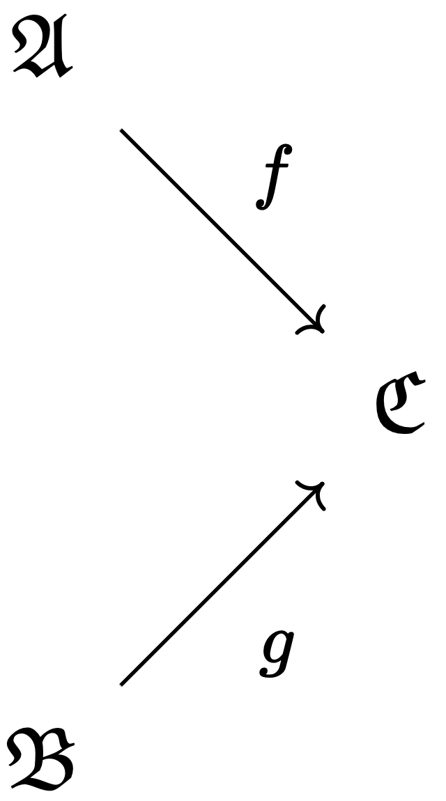
증명. 이 글의 표기법을 따라, 언어 $L_\mathfrak{A}$의 이론 $E(\mathfrak{A})$와 언어 $L’_\mathfrak{B}$의 이론 $E(\mathfrak{B})$를 생각하자. $T = E(\mathfrak{A}) \cup E(\mathfrak{B})$는 언어 $\mathcal{L}’_{\mathfrak{AB}} = \mathcal{L}_\mathfrak{A} \cup \mathcal{L}’_\mathfrak{B}$의 이론이다. $T$가 모델 $\mathfrak{C}$를 가짐을 보이자.

만약 $T$가 모델이 없다면 $T$는 모순적이다. 따라서 콤팩트성 정리에 의해 어떤 $\mathcal{L}$-논리식 $\phi$와 $\mathcal{L}’$-논리식 $\psi$가 존재하여, 적절한 $\lbrace a_i \rbrace \subset \mathcal{L}_\mathfrak{A}$, $\lbrace b_j \rbrace \subset \mathcal{L}_\mathfrak{B}$에 대해,

\[\lbrace \phi(a_1, \dots, a_n), \psi(b_1, \dots, b_m) \rbrace\]

이 모델을 가지지 않는다. $\mathfrak{B} \vDash \psi(b_1, \dots, b_m)$이므로, $\mathfrak{B} \vDash \phi(a_1, \dots, a_n)$를 만족하도록 상수 $a_1, \dots, a_n$을 $\mathfrak{B}$의 정의역에 대응시키는 방법이 존재하지 않아야 한다. 즉,

\[\mathfrak{B} \not\vDash \exists x_1, \dots x_n \; \phi(x_1, \dots, x_n)\]

그런데 $\mathfrak{B}$의 $\mathcal{L}$-퇴화가 $\mathfrak{A}$와 초등적으로 동등하며, 위 식의 우변이 $\mathcal{L}$-문장이고, $\mathfrak{A}$가 해당 문장을 만족하므로 이는 모순이다. 따라서 $T$는 모델 $\mathfrak{C}$를 가진다. 그리고 $\mathfrak{C}$는 $E(\mathfrak{A})$와 $E(\mathfrak{B})$의 모델이므로, $\mathfrak{A}$와 $\mathfrak{B}$는 $\mathfrak{C}$로 자연스럽게 초등적으로 임베딩된다. ■

로빈슨 건전성 정리_{Robinson consistency theorem}

정리. $\mathcal{L} = \mathcal{L}_1 \cap \mathcal{L}_2$라고 하자. $T$가 $\mathcal{L}$의 (의미론적으로) 완전한 이론이고, $T_1$과 $T_2$가 각각 $T$를 확장하는 건전한 $\mathcal{L}_1, \mathcal{L}_2$ 이론일 때, $T_1 \cup T_2$는 $\mathcal{L}_1 \cup \mathcal{L}_2$ 이론으로서 건전하다.

증명. $T_1 \cup T_2$의 모델을 구축하면 정리가 보여진다.

$T_1, T_2$가 각각 건전하므로, 모델 $\mathfrak{A}_0, \mathfrak{B}_0$를 가진다. $T = T_1 \cap T_2$가 완전하므로, $\mathcal{L}$-퇴화로서의 $\mathfrak{A}_0$와 $\mathfrak{B}_0$는 초등적으로 동등하다. 따라서 초등적 병합 성질에 의해, $\mathcal{L}$-초등적 임베딩 $f_0$와 $\mathcal{L}_2$-초등적 임베딩 $h_0$가 존재하여 다음이 성립한다.

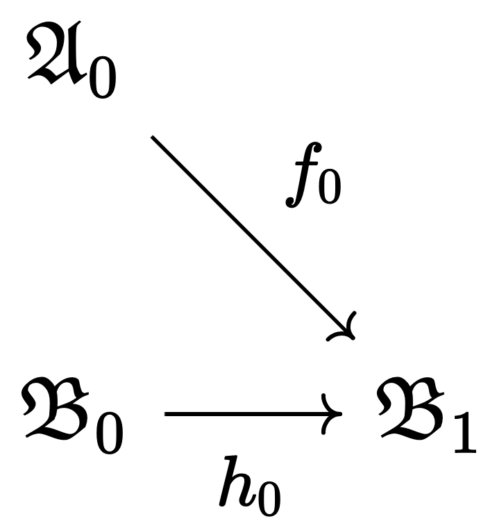
이제 $\mathfrak{B}_1$의 $\mathcal{L}$-퇴화를 생각해 보면, 이는 $\mathfrak{A}_0$와 초등적으로 동등하므로, 다시 초등적 병합 성질에 의해 $\mathcal{L}$-초등적 임베딩 $g_0$와 $\mathcal{L}_1$-초등적 임베딩 $k_0$가 존재하여 다음이 성립한다.

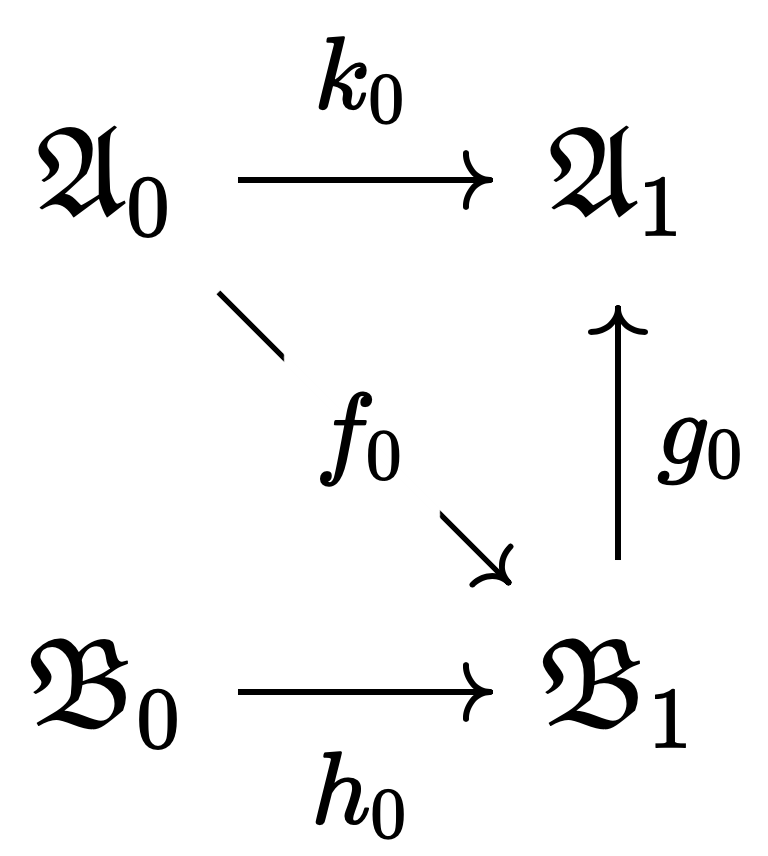
이 과정을 반복하여 다음의 구조 유도계_{directed system of structures}를 얻는다.

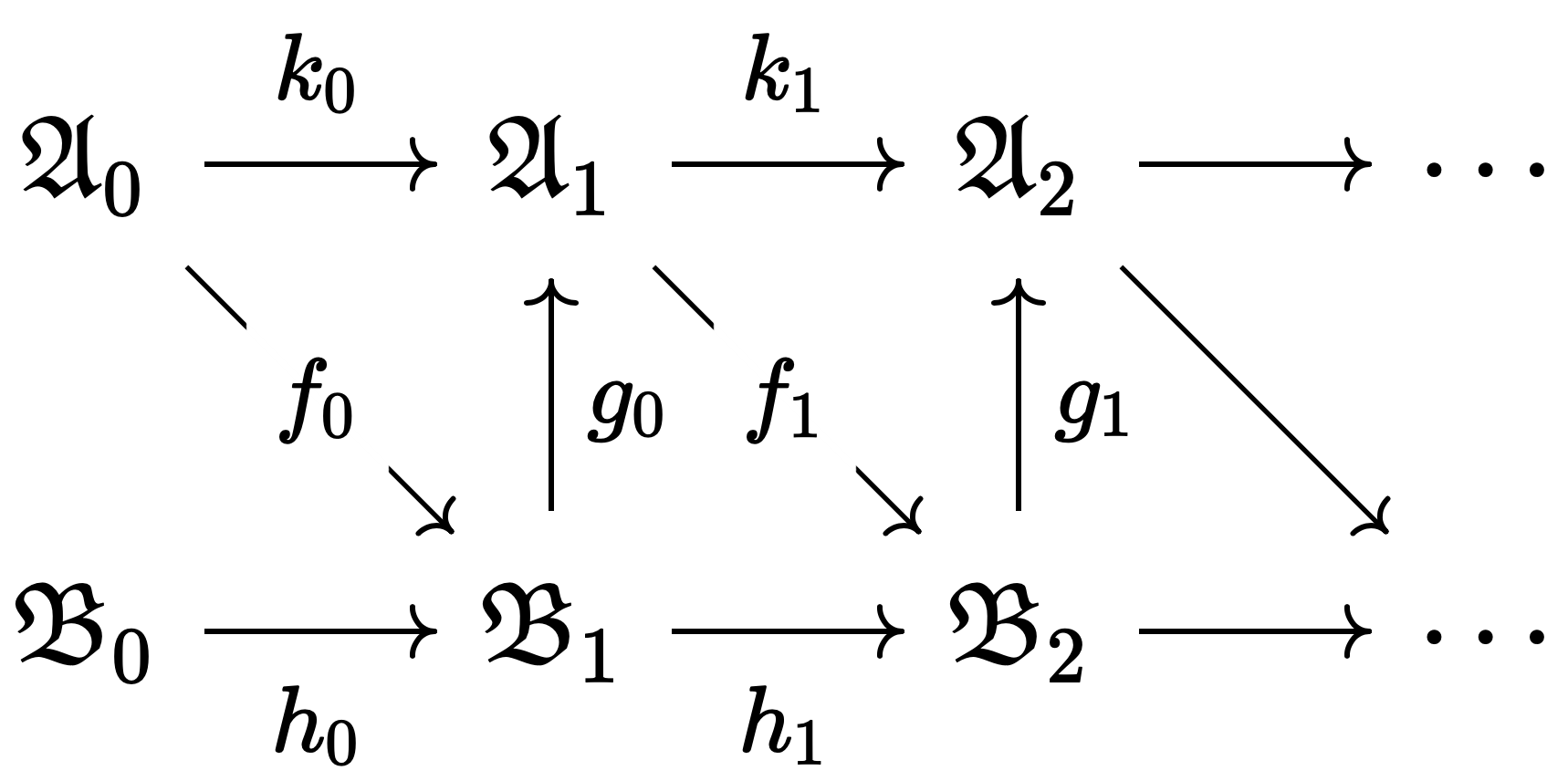
사상	성질
$f, g$	$\mathcal{L}$-초등적 임베딩
$k$	$\mathcal{L}_1$-초등적 임베딩
$h$	$\mathcal{L}_2$-초등적 임베딩

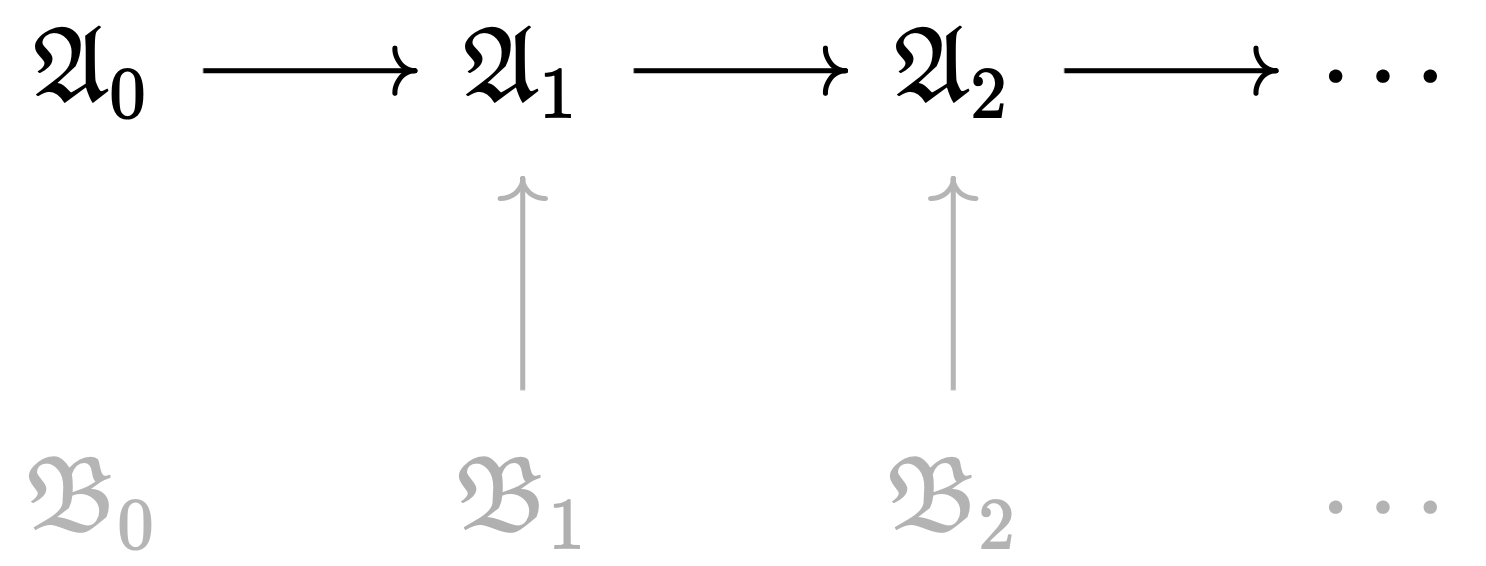
위 유도계의 모든 모델을 $\mathcal{L}$로 퇴화시키면 $\mathcal{L}$-구조 유도계를 얻는다. 해당 유도계의 쌍대극한_colimit을 $\mathfrak{C}$라고 하자. $\mathfrak{C}$는 다음의 $\lbrace \mathfrak{A}_i \rbrace $로 이루어진 유도계의 쌍대극한이기도 하다. 회색으로 표시된 원 유도계의 일부는 모두 $\lbrace \mathfrak{A}_i \rbrace $ 중 하나로 투사되기 때문이다. 따라서 $\mathfrak{C}$는 $\mathfrak{A}_0$를 초등적으로 임베딩하는 $\mathcal{L}_1$ 구조이다.

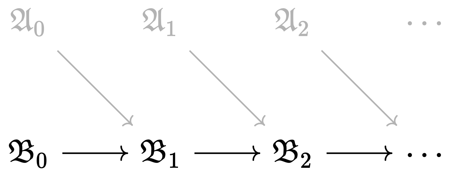
같은 이유로 $\mathfrak{C}$는 다음의 $\lbrace \mathfrak{B}_i \rbrace $로 이루어진 유도계의 쌍대극한이기도 하다. 따라서 $\mathfrak{C}$는 $\mathfrak{B}_0$를 초등적으로 임베딩하는 $\mathcal{L}_2$ 구조이다.

즉, $\mathfrak{C}$는 $\mathfrak{A}$와 $\mathfrak{B}$를 모두 임베딩하며, 이로부터 $T_1 \cup T_2$의 모델임이 보여졌다. ■

크레이그 보간 정리_{Craig interpolation theorem}

정리. $\mathcal{L}$-문장 $\phi, \psi$에 대해 $\phi \vDash \psi$라면, 어떤 $\mathcal{L}$-문장 $\theta$가 존재하여 $\phi \vDash \theta, \theta \vDash \psi$이다. 또한, $\theta$에 포함된 비논리 기호(상수, 술어, 함수)는 $\phi$와 $\psi$에 공통적으로 포함된다.

$\theta$를 $\phi$와 $\psi$의 크레이그 보간이라고 부른다.

증명. 귀류법으로 증명한다. 크레이그 보간이 존재하지 않는다고 가정하자. 그러면 $\phi$는 모델을 가진다. 만약 $\phi$가 모델을 가지지 않는다면 $\perp$가 $\phi, \psi$의 크레이그 보간이기 때문이다. 또한 $\lnot \psi$도 모델을 가진다. 그렇지 않다면 $\top$가 크레이그 보간이기 때문이다.

$\mathcal{L}’$을 $\phi$와 $\psi$에 공통적으로 포함되는 비논리 기호들로 이루어진 언어라고 하자. $\Gamma$를, $\phi \vDash \sigma$이거나 $\lnot \psi \vDash \sigma$인 $\mathcal{L}’$-문장 $\sigma$의 집합이라고 하자.

$\Gamma \cup \lbrace \phi \rbrace $는 무모순적임을 보이자. 만약 모순적이라면, 콤팩트성 정리에 의해 어떤 $\mathcal{L}’$-문장 $\sigma_1, \sigma_2$가 존재하여 $\phi \vDash \sigma_1, \lnot\psi \vDash \sigma_2$이고 $\lbrace \sigma_1, \sigma_2, \phi \rbrace $가 모순적이다. 그런데 $\phi \vDash \sigma_1$이므로 $\phi \vDash \lnot\sigma_2$이다. 대우법에 의해 $\lnot\psi\ \vDash \sigma_2$로부터 $\lnot\sigma_2 \vDash \psi$가 따라 나온다. 즉, $\sigma_2$는 $\phi, \psi$의 크레이그 보간이다. 이는 가정에 모순된다.

따라서 $\Gamma \cup \lbrace \phi \rbrace $는 무모순적이며, 같은 이유로 $\Gamma \cup \lbrace \lnot\psi \rbrace $ 또한 무모순적이다. 이제 초른의 보조정리를 적용하여, $\overline{\Gamma}$를 다음 $\mathcal{L}’$-이론들의 순서의 극대로 정의한다.

\[\{ \Gamma' : \Gamma \subseteq \Gamma', \Gamma' \cup \{\phi\} \text{ and } \Gamma' \cup \{\lnot \psi\} \text{ are consistent} \}\]

$\overline{\Gamma}$는 완전함을 보이자. 만약 $\overline{\Gamma}$가 완전하지 않다면, 어떤 $\mathcal{L}’$-문장 $\sigma$가 존재하여 $\sigma \notin \overline{\Gamma}$이고, $\overline{\Gamma} \cup \lbrace \sigma, \phi \rbrace $ 또는 $\overline{\Gamma} \cup \lbrace \sigma, \lnot \psi \rbrace $가 무모순적이다.

전자의 경우, 콤팩트성 정리에 의해 어떤 $\overline{\Gamma}$의 문장 $\theta$가 존재하여 $\phi \vDash \theta \rightarrow \lnot \sigma$이다. $\Gamma$의 정의에 의해 $\theta \rightarrow \lnot \sigma \in \Gamma \subseteq \overline{\Gamma}$이다. 따라서 $\overline{\Gamma} \cup \lbrace \sigma, \phi \rbrace $는 $\lnot\phi$를 증명한다. 이는 모순이다. 후자의 경우에도 마찬가지 모순이 발생한다. 따라서 $\overline{\Gamma}$는 완전하다.

$\overline{\Gamma}$가 완전하고, $\overline{\Gamma} \cup \lbrace \phi \rbrace , \overline{\Gamma} \cup \lbrace \lnot\psi \rbrace $가 건전하므로, 로빈슨 건전성 정리에 의해 $\overline{\Gamma} \cup \lbrace \phi, \lnot \psi \rbrace $가 건전하다. 그런데 이는 $\phi \vDash \psi$에 모순된다. 따라서 귀류법에 의해 $\phi, \psi$는 크레이그 보간을 가진다. ■

베스 정의 가능성 정리_{Beth definability theorem}

언어 $\mathcal{L}$과, $\mathcal{L}$에 포함되어 있지 않은 술어 $P$를 생각하자. $T$가 $\mathcal{L} \cup \lbrace P \rbrace $의 이론이라고 하자. $T$를 만족하는 $\mathcal{L}$의 구조 $\mathfrak{A}$를 $\mathcal{L} \cup \lbrace P \rbrace $로 확장하는 방법이 유일할 때, $T$가 $P$를 암시적으로 정의_{implicitly define}한다고 한다.

이는 다음과 같이 말할 수도 있다. $T(P’)$가 $T$에서 등장하는 모든 $P$를 $P’$으로 바꾼 $\mathcal{L} \cup \lbrace P’ \rbrace $ 이론이라고 하자. $T$가 $P$를 암시적으로 정의한다는 것은 다음이 성립한다는 것이다.

\[T \cup T(P') \vDash \forall x_1, \dots, x_n \; P(x_1, \dots, x_n) \leftrightarrow P'(x_1, \dots, x_n)\]

반면 $T$가 $P$를 명시적으로 정의_{explicitly define}한다는 것은 다음을 만족시키는 $\mathcal{L}$-논리식 $\phi$가 존재한다는 것이다.

\[T \vDash \forall x_1, \dots, x_n \; P(x_1, \dots, x_n) \leftrightarrow \phi(x_1, \dots, x_n)\]

예를 들어 보자. $\mathcal{L} = (0, S, +, \cdot)$의 이론 $\mathsf{PA}$에 술어 $P(x, y)$에 관한 공리를 추가한 다음의 이론을 $T$라고 하자.

\[T = \mathsf{PA} \cup \Big\{ \forall x, y \big[ P(x, y) \rightarrow x + y = S(0) \big] \Big\}\]

$T(P’)$은 다음과 같다.

\[T(P') = \mathsf{PA} \cup \Big\{ \forall x, y \big[ P'(x, y) \rightarrow x + y = S(0) \big] \Big\}\]

$T$가 $P$를 암묵적으로 정의한다는 것은 다음이 성립한다는 것이다.

\[T \cup T(P') \vDash \forall x, y \big[ P(x, y) \leftrightarrow P'(x, y) \big]\]

이는 귀납 공리꼴로부터 자연스럽게 따라 나온다. 그런데 $P$는 다음과 같이 $T$에서 명시적으로 정의될 수도 있다.

\[\begin{gather} T \vDash \forall x, y \big[ P(x, y) \leftrightarrow \phi(x, y) \big] \\\\ \text{where}\\\\ \phi(x, y) : \forall z \big[ x + z = S(0) \rightarrow z = y \big] \end{gather}\]

이는 우연이 아니다.

정리. 언어 $\mathcal{L}$에 대해, $\mathcal{L} \cup \lbrace P \rbrace $의 이론 $T$가 $P$를 암시적으로 정의하면, $T$는 $P$를 명시적으로 정의한다.

증명. $P$가 $n$항 술어라고 하자. $\mathcal{L}$에 새로운 상수 $c_1, \dots, c_n$을 추가한 언어를 $\mathcal{L}’$이라고 하자. $T$가 $P$를 암시적으로 정의하므로,

\[T \cup T(P') \vDash P(c_1, \dots, c_n) \rightarrow P'(c_1, \dots, c_n)\]

이다. 콤팩트성 정리에 의해 어떤 $\mathcal{L} \cup \lbrace P \rbrace $ 문장 $\psi$가 존재하여, $T \vdash \psi$이고 다음이 성립한다.

\[\psi \land \psi(P') \vDash P(c_1, \dots, c_n) \rightarrow P'(c_1, \dots, c_n)\]

함축 원리를 이용하여 이항하면 다음과 같다.

\[\psi \land P(c_1, \dots, c_n) \vDash \psi(P') \rightarrow P'(c_1, \dots, c_n)\]

좌변은 $\mathcal{L}’ \cup \lbrace P \rbrace $의 문장이고, 우변은 $\mathcal{L}’ \cup \lbrace P’ \rbrace $의 문장이다. 따라서 크레이그 보간 정리에 의해 $\mathcal{L}$-논리식 $\theta$가 존재하여 다음이 성립한다.

\[\begin{gather} \psi \land P(c_1, \dots, c_n) \vDash \theta(c_1, \dots, c_n), \\\\ \theta(c_1, \dots, c_n) \vDash \psi(P') \rightarrow P'(c_1, \dots, c_n) \end{gather}\]

다시 이항하고 $P’$을 $P$로 치환하면,

\[\begin{gather} \psi \vDash P(c_1, \dots, c_n) \rightarrow \theta(c_1, \dots, c_n), \\\\ \psi \vDash \theta(c_1, \dots, c_n) \rightarrow P(c_1, \dots, c_n) \end{gather}\]

따라서 $\theta$는 $P$를 명시적으로 정의한다. ■

Robinson, Craig, and Beth's Theorems

08 May 2025

This post was originally written in Korean, and has been machine translated into English. It may contain minor errors or unnatural expressions. Proofreading will be done in the near future.

Elementary Amalgamation Property

Theorem. Let $\mathfrak{A}$ be an $\mathcal{L}$-structure and $\mathfrak{B}$ be an $\mathcal{L}’$-structure such that the $\mathcal{L}$-reduct of $\mathfrak{B}$ is elementarily equivalent to $\mathfrak{A}$. Then there exists an $\mathcal{L}’$-structure $\mathfrak{C}$ such that $f: \mathfrak{A} \to \mathfrak{C}$ is an elementary embedding in $\mathcal{L}$ and $g: \mathfrak{B} \to \mathfrak{C}$ is an elementary embedding in $\mathcal{L}’$.

Proof. Following the notation of this post, consider the theory $E(\mathfrak{A})$ in language $L_\mathfrak{A}$ and the theory $E(\mathfrak{B})$ in language $L’\mathfrak{B}$. Let $T = E(\mathfrak{A}) \cup E(\mathfrak{B})$ be a theory in the language $\mathcal{L}’{\mathfrak{AB}} = \mathcal{L}\mathfrak{A} \cup \mathcal{L}’\mathfrak{B}$. We shall show that $T$ has a model $\mathfrak{C}$.

Suppose $T$ has no model. Then $T$ is inconsistent. By the compactness theorem, there exist some $\mathcal{L}$-formula $\phi$ and $\mathcal{L}’$-formula $\psi$ such that for appropriate ${a_i} \subset \mathcal{L}\mathfrak{A}$ and ${b_j} \subset \mathcal{L}\mathfrak{B}$,

\[\{\phi(a_1, \dots, a_n), \psi(b_1, \dots, b_m)\}\]

has no model. Since $\mathfrak{B} \vDash \psi(b_1, \dots, b_m)$, there must be no way to assign the constants $a_1, \dots, a_n$ to elements of the domain of $\mathfrak{B}$ such that $\mathfrak{B} \vDash \phi(a_1, \dots, a_n)$. That is,

\[\mathfrak{B} \not\vDash \exists x_1, \dots x_n \; \phi(x_1, \dots, x_n)\]

However, since the $\mathcal{L}$-reduct of $\mathfrak{B}$ is elementarily equivalent to $\mathfrak{A}$, and the right-hand side above is an $\mathcal{L}$-sentence that is satisfied by $\mathfrak{A}$, this yields a contradiction. Therefore, $T$ has a model $\mathfrak{C}$. Since $\mathfrak{C}$ is a model of both $E(\mathfrak{A})$ and $E(\mathfrak{B})$, both $\mathfrak{A}$ and $\mathfrak{B}$ are naturally elementarily embedded into $\mathfrak{C}$. ■

Robinson Consistency Theorem

Theorem. Let $\mathcal{L} = \mathcal{L}_1 \cap \mathcal{L}_2$. Suppose $T$ is a (semantically) complete theory in $\mathcal{L}$, and $T_1$ and $T_2$ are consistent theories in $\mathcal{L}_1$ and $\mathcal{L}_2$ respectively, each extending $T$. Then $T_1 \cup T_2$ is consistent as a theory in $\mathcal{L}_1 \cup \mathcal{L}_2$.

Proof. It suffices to construct a model of $T_1 \cup T_2$.

Since $T_1$ and $T_2$ are consistent, they have models $\mathfrak{A}_0$ and $\mathfrak{B}_0$ respectively. Since $T = T_1 \cap T_2$ is complete, the $\mathcal{L}$-reducts of $\mathfrak{A}_0$ and $\mathfrak{B}_0$ are elementarily equivalent. Therefore, by the elementary amalgamation property, there exist an $\mathcal{L}$-elementary embedding $f_0$ and an $\mathcal{L}_2$-elementary embedding $h_0$ such that the following holds:

Now considering the $\mathcal{L}$-reduct of $\mathfrak{B}_1$, this is elementarily equivalent to $\mathfrak{A}_0$, so again by the elementary amalgamation property, there exist an $\mathcal{L}$-elementary embedding $g_0$ and an $\mathcal{L}_1$-elementary embedding $k_0$ such that the following holds:

Repeating this process, we obtain the following directed system of structures:

Map	Property
$f, g$	$\mathcal{L}$-elementary embedding
$k$	$\mathcal{L}_1$-elementary embedding
$h$	$\mathcal{L}_2$-elementary embedding

Reducing all models in the above directed system to $\mathcal{L}$ gives an $\mathcal{L}$-structure directed system. Let $\mathfrak{C}$ be the colimit of this directed system. $\mathfrak{C}$ is also the colimit of the directed system consisting of ${\mathfrak{A}_i}$, since the parts of the original directed system shown in grey all project to one of the ${\mathfrak{A}_i}$. Therefore, $\mathfrak{C}$ is an $\mathcal{L}_1$-structure that elementarily embeds $\mathfrak{A}_0$.

For the same reason, $\mathfrak{C}$ is also the colimit of the directed system consisting of ${\mathfrak{B}_i}$. Therefore, $\mathfrak{C}$ is an $\mathcal{L}_2$-structure that elementarily embeds $\mathfrak{B}_0$.

That is, $\mathfrak{C}$ embeds both $\mathfrak{A}$ and $\mathfrak{B}$, from which it follows that it is a model of $T_1 \cup T_2$. ■

Craig Interpolation Theorem

Theorem. For $\mathcal{L}$-sentences $\phi$ and $\psi$, if $\phi \vDash \psi$, then there exists an $\mathcal{L}$-sentence $\theta$ such that $\phi \vDash \theta$ and $\theta \vDash \psi$. Moreover, the non-logical symbols (constants, predicates, functions) contained in $\theta$ are those common to both $\phi$ and $\psi$.

$\theta$ is called a Craig interpolant of $\phi$ and $\psi$.

Proof. We prove by contradiction. Suppose no Craig interpolant exists. Then $\phi$ has a model, for if $\phi$ had no model, then $\perp$ would be a Craig interpolant of $\phi$ and $\psi$. Also, $\lnot \psi$ has a model, for otherwise $\top$ would be a Craig interpolant.

Let $\mathcal{L}’$ be the language consisting of the non-logical symbols common to both $\phi$ and $\psi$. Let $\Gamma$ be the set of $\mathcal{L}’$-sentences $\sigma$ such that either $\phi \vDash \sigma$ or $\lnot \psi \vDash \sigma$.

We show that $\Gamma \cup {\phi}$ is consistent. Suppose it is inconsistent. Then by the compactness theorem, there exist $\mathcal{L}’$-sentences $\sigma_1$ and $\sigma_2$ such that $\phi \vDash \sigma_1$, $\lnot\psi \vDash \sigma_2$, and ${\sigma_1, \sigma_2, \phi}$ is inconsistent. Since $\phi \vDash \sigma_1$, we have $\phi \vDash \lnot\sigma_2$. By contraposition, from $\lnot\psi \vDash \sigma_2$ we obtain $\lnot\sigma_2 \vDash \psi$. Thus $\lnot\sigma_2$ is a Craig interpolant of $\phi$ and $\psi$, contradicting our assumption.

Therefore, $\Gamma \cup {\phi}$ is consistent, and by the same reasoning, $\Gamma \cup {\lnot\psi}$ is also consistent. Now applying Zorn’s lemma, define $\overline{\Gamma}$ as the maximum of the following ordered set of $\mathcal{L}’$-theories:

\[\{ \Gamma' : \Gamma \subseteq \Gamma', \Gamma' \cup \{\phi\} \text{ and } \Gamma' \cup \{\lnot \psi\} \text{ are consistent} \}\]

We show that $\overline{\Gamma}$ is complete. Suppose $\overline{\Gamma}$ is not complete. Then there exists an $\mathcal{L}’$-sentence $\sigma$ such that $\sigma \notin \overline{\Gamma}$, and either $\overline{\Gamma} \cup {\sigma, \phi}$ or $\overline{\Gamma} \cup {\sigma, \lnot \psi}$ is consistent.

In the former case, by the compactness theorem, there exists a sentence $\theta$ in $\overline{\Gamma}$ such that $\phi \vDash \theta \rightarrow \lnot \sigma$. By the definition of $\Gamma$, we have $\theta \rightarrow \lnot \sigma \in \Gamma \subseteq \overline{\Gamma}$. Therefore, $\overline{\Gamma} \cup {\sigma, \phi}$ proves $\lnot\phi$, which is a contradiction. The latter case yields a similar contradiction. Therefore, $\overline{\Gamma}$ is complete.

Since $\overline{\Gamma}$ is complete and $\overline{\Gamma} \cup {\phi}$ and $\overline{\Gamma} \cup {\lnot\psi}$ are consistent, by Robinson’s consistency theorem, $\overline{\Gamma} \cup {\phi, \lnot \psi}$ is consistent. But this contradicts $\phi \vDash \psi$. Therefore, by contradiction, $\phi$ and $\psi$ have a Craig interpolant. ■

Beth Definability Theorem

Consider a language $\mathcal{L}$ and a predicate $P$ not contained in $\mathcal{L}$. Let $T$ be a theory in $\mathcal{L} \cup {P}$. We say that $T$ implicitly defines $P$ when there is a unique way to extend any $\mathcal{L}$-structure $\mathfrak{A}$ satisfying $T$ to $\mathcal{L} \cup {P}$.

This can also be stated as follows. Let $T(P’)$ be the theory in $\mathcal{L} \cup {P’}$ obtained by replacing every occurrence of $P$ in $T$ with $P’$. Then $T$ implicitly defines $P$ if and only if the following holds:

\[T \cup T(P') \vDash \forall x_1, \dots, x_n \; P(x_1, \dots, x_n) \leftrightarrow P'(x_1, \dots, x_n)\]

On the other hand, $T$ explicitly defines $P$ if there exists an $\mathcal{L}$-formula $\phi$ satisfying:

\[T \vDash \forall x_1, \dots, x_n \; P(x_1, \dots, x_n) \leftrightarrow \phi(x_1, \dots, x_n)\]

For example, consider the following theory $T$, which adds axioms concerning a predicate $P(x, y)$ to the theory $\mathsf{PA}$ in the language $\mathcal{L} = (0, S, +, \cdot)$:

\[T = \mathsf{PA} \cup \Big\{ \forall x, y \big[ P(x, y) \rightarrow x + y = S(0) \big] \Big\}\]

$T(P’)$ is as follows:

\[T(P') = \mathsf{PA} \cup \Big\{ \forall x, y \big[ P'(x, y) \rightarrow x + y = S(0) \big] \Big\}\]

That $T$ implicitly defines $P$ means the following holds:

\[T \cup T(P') \vDash \forall x, y \big[ P(x, y) \leftrightarrow P'(x, y) \big]\]

This follows naturally from the induction axiom schema. But $P$ can also be explicitly defined in $T$ as follows:

\[\begin{gather} T \vDash \forall x, y \big[ P(x, y) \leftrightarrow \phi(x, y) \big] \\\\ \text{where}\\\\ \phi(x, y) : \forall z \big[ x + z = S(0) \rightarrow z = y \big] \end{gather}\]

This is no coincidence.

Theorem. For a language $\mathcal{L}$, if a theory $T$ in $\mathcal{L} \cup {P}$ implicitly defines $P$, then $T$ explicitly defines $P$.

Proof. Suppose $P$ is an $n$-ary predicate. Let $\mathcal{L}’$ be the language obtained by adding new constants $c_1, \dots, c_n$ to $\mathcal{L}$. Since $T$ implicitly defines $P$, we have:

\[T \cup T(P') \vDash P(c_1, \dots, c_n) \rightarrow P'(c_1, \dots, c_n)\]

By the compactness theorem, there exists an $\mathcal{L} \cup {P}$-sentence $\psi$ such that $T \vdash \psi$ and the following holds:

\[\psi \land \psi(P') \vDash P(c_1, \dots, c_n) \rightarrow P'(c_1, \dots, c_n)\]

Using the deduction theorem and rearranging:

\[\psi \land P(c_1, \dots, c_n) \vDash \psi(P') \rightarrow P'(c_1, \dots, c_n)\]

The left-hand side is a sentence in $\mathcal{L}’ \cup {P}$, and the right-hand side is a sentence in $\mathcal{L}’ \cup {P’}$. Therefore, by Craig’s interpolation theorem, there exists an $\mathcal{L}’$-formula $\theta$ such that:

\[\begin{gather} \psi \land P(c_1, \dots, c_n) \vDash \theta(c_1, \dots, c_n), \\\\ \theta(c_1, \dots, c_n) \vDash \psi(P') \rightarrow P'(c_1, \dots, c_n) \end{gather}\]

Rearranging again and substituting $P$ for $P’$:

\[\begin{gather} \psi \vDash P(c_1, \dots, c_n) \rightarrow \theta(c_1, \dots, c_n), \\\\ \psi \vDash \theta(c_1, \dots, c_n) \rightarrow P(c_1, \dots, c_n) \end{gather}\]

Therefore, $\theta$ explicitly defines $P$. ■

정칙 기수와 특이 기수, 그리고 도달 불가능 기수

04 May 2025

이 글에서 $\kappa$는 무한 기수이다. 또한, 기수를 초기 서수_{initial ordinal}로 정의하는 방식을 택한다(이 글의 3번). 이에 따라 모든 기수는 서수이기도 하다.

정의. $\theta$가 $\kappa$보다 작은 극한 서수라고 하자. 각 $\nu$에 대해 $\alpha_\nu < \kappa$인 증가하는 서수열 $\langle \alpha_\nu : \nu < \theta \rangle$에 대하여, 언제나 $\lim_{\nu \to \theta} \alpha_\nu < \kappa$일 때, $\kappa$를 정칙 기수_{regular cardinal}라고 한다. 정칙 기수가 아닌 기수를 특이 기수_{singular cardinal}라고 한다.

Remark. $\alpha_\nu$와 $\theta$는 일반적으로 기수가 아니라 서수이다.

예를 들어 $\aleph_0$는 정칙 기수이다. $\aleph_0$개보다 적은 개수의 — 즉, 유한한 — $\aleph_0$보다 작은 기수들 — 즉, 자연수 — 의 상한은 $\aleph_0$에 달하지 않기 때문이다.

반면 $\aleph_\omega$는 특이 기수이다. 다음 기수열에서 각각의 기수는 $\aleph_\omega$보다 작고, 기수열의 길이 또한 $\aleph_0 < \aleph_\omega$이지만, 그 상한은 $\aleph_\omega$이기 때문이다.

\[\aleph_0 \quad \aleph_1 \quad \aleph_2 \quad \aleph_3 \quad \cdots\]

정리. (특이 기수 판별법) $\kappa$가 특이 기수일 필요충분조건은 $\kappa$가 $\kappa$개보다 적은 개수의 $\kappa$보다 작은 기수들의 합일 것이다. 즉, $|I| < \kappa$, $\kappa_i < \kappa \;(\forall i \in I)$에 대하여,

\[\sum_{i \in I} \kappa_i = \kappa\]

Remark. $\kappa_i$는 일반적인 서수가 아닌 기수이다. 그리고 $\sum$은 서수 덧셈이 아니라 기수 덧셈이다.

증명.

($\Rightarrow$) $\kappa$가 특이 기수라면 어떤 서수열 $\langle \alpha_\nu : \nu < \theta\rangle$이 존재하여,

\[\lim_{\nu \to \theta} \alpha_\nu = \sup \alpha_\nu = \bigcup_{\nu < \theta}\alpha_\nu = \kappa\]

이다. 일반적으로 서수 $\alpha$는 자기보다 작은 서수 $\beta < \alpha$들의 합집합이다. 따라서 다음이 성립한다.

\[\kappa = \bigcup_{\nu < \theta}\alpha_\nu = \bigcup_{\nu < \theta}\left( \alpha_\nu - \bigcup_{\xi < \nu} \alpha_\xi \right)\]

$A_\nu = \alpha_\nu - \bigcup_{\xi < \nu} \alpha_\xi$라고 하자. $A_\nu$는 더이상 서수가 아니지만 그건 중요하지 않다. 중요한 것은 $\lbrace A_\nu \rbrace $가 쌍으로 서로소라는 것이다. 따라서 $\kappa_\nu = |A_\nu|$라고 하면 기수 덧셈의 정의에 의해,

\[\sum_{\nu < \theta} \kappa_\nu = \left| \bigcup_{\nu < \theta} A_\nu \right| = \kappa\]

이다.

($\Leftarrow$) $\kappa = \sum_{i \in I}\kappa_i$라고 하자. $|I| = \lambda$라고 하면 기수 덧셈의 성질에 의해 $\kappa = \lambda \cdot \sup \kappa_i$이다. $\lambda < \kappa$이므로, 기수 곱셈의 성질에 의해 $\kappa = \sup \kappa_i$이다. 각 $i \in I$에 대해 $\kappa_i < \kappa$인데 $\sup \kappa_i = \kappa$이므로, 초한귀납법을 통해 증가하는 기수열

\[\langle \kappa_\nu : \kappa_\nu = \kappa_i \text{ for some } i \in I, \nu < \theta\rangle\]

을 구축할 수 있으며, $\theta \leq \lambda$이므로 정리가 보여졌다. ■

정의. 어떤 $\alpha \in \mathrm{Ord}$에 대해 $\kappa = \aleph_{\alpha + 1}$일 때, $\kappa$를 계승 기수_{successor cardinal}라고 한다. 계승 기수가 아닌 기수를 극한 기수_{limit cardinal}라고 한다.

정리. 모든 계승 기수는 정칙이다.

증명. $\kappa = \aleph_{\alpha + 1}$이라고 하자. $\kappa$가 특이 기수라면, 특이 기수 판별법에 의해 $\kappa = \sum_{i \in I} \kappa_i$이며 $\kappa_i, |I| < \kappa$이다. 이는 $\kappa_i , |I| \leq \aleph_\alpha$와 같다. 그런데

\[\sum_{i \in I} \kappa_i \leq \sum_{i \in I} \aleph_\alpha = |I| \cdot \aleph_\alpha \leq \aleph_\alpha \cdot \aleph_\alpha = \aleph_\alpha < \kappa\]

이므로 모순이다. ■

따라서 모든 특이 기수는 극한 기수이다. 그러나 모든 극한 기수가 특이 기수인 것은 아니다. $\aleph_0$는 정칙인 극한 기수이기 때문이다. 그러나 $\aleph_0$ 이외에 정칙인 극한 기수가 존재할까?

정의. 비가산 정칙 극한 기수를 도달 불가능 기수_{inaccessible cardinal}라고 한다.¹

$\aleph_\alpha$가 도달 불가능 기수라고 하자. 다음의 증가 기수열의 극한은 $\aleph_\alpha$이다.

\[\langle \aleph_\beta : \beta < \alpha \rangle : \aleph_0 \quad \aleph_1 \quad \aleph_2 \quad \cdots \quad \to \aleph_\alpha\]

따라서 $\aleph_\alpha$가 정칙이기 위해서는 위 기수열의 길이인 $\alpha$가 $\aleph_\alpha$보다 작아서는 안 된다. 그런데 $\alpha \leq \aleph_\alpha$이므로, $\alpha = \aleph_\alpha$임이 따라 나온다.

정리. $\aleph_\alpha$가 도달 불가능할 필요조건은 $\alpha = \aleph_\alpha$인 것이다.

이는 $\alpha$가 무지막지하게 큰 기수임을 시사한다. 일례로 다음의 기수열 $\langle \alpha_n : n \in \omega \rangle$을 보자.

\[\alpha_0 = \aleph_0, \alpha_{n + 1} = \aleph_{\alpha_n}\]

위 기수열의 상한을 $\kappa$라고 하자. 상한의 정의에 의해 $\lambda < \kappa$라면 $\alpha_n > \lambda$인 $n$이 존재한다. 따라서 $\aleph_\lambda = \alpha_{n+1} < \kappa$이며,

\[\aleph_\kappa = \sum_{\lambda < \kappa} \aleph_\lambda \leq \sum_{\lambda < \kappa} \kappa = \kappa\]

이다. 다시 말해, $\alpha = \aleph_\alpha$를 만족하는 기수는 적어도 다음에 비견되는 크기를 가진다.

\[\kappa = \aleph_{\aleph_{\aleph_{\aleph_{\ddots}}}}\]

여기서 집고 넘어갈 점이 있다. 비록 $\kappa$가 $\kappa = \aleph_\kappa$를 보이긴 했지만, $\kappa$가 도달 불가능함을 보인 것은 아니다. 오히려 $\kappa$는 특이 기수이다. 길이가 $\omega$인 기수열 $\alpha_n$의 극한이기 때문이다.

사실 도달 불가능 기수의 존재성은 ZFC와 독립적이다.

정리. 도달 불가능 기수의 존재성은 ZFC와 독립이다.

따라서 도달 불가능 기수의 존재는 공리로서 가정해야 한다. 도달 불가능 기수의 존재를 가정하는 부류의 공리들을 큰 기수 공리_{large cardinal axioms}라고 부르며, 이와 관련된 연구는 집합론의 중요한 부분을 이룬다.

---

1. 엄밀히 말해 이는 약한 도달 불가능 기수_{weakly inaccessible cardinal}에 해당한다. $\kappa$가 강한 도달 불가능 기수_{strongly inaccessible cardinal}라는 것은 $\kappa$가 약한 도달 불가능 기수이며, 추가로 $\lambda < \kappa$일 때 $2^\lambda < \kappa$인 것이다. 연속체 가설을 인정할 때 약한 도달 불가능성과 강한 도달 불가능성은 동치이다.

Regular Cardinals, Singular Cardinals, and Inaccessible Cardinals

04 May 2025

This post was originally written in Korean, and has been machine translated into English. It may contain minor errors or unnatural expressions. Proofreading will be done in the near future.

In this article, $\kappa$ denotes an infinite cardinal. Moreover, we adopt the approach of defining cardinals as initial ordinals (see method 3 in this post). Accordingly, every cardinal is also an ordinal.

Definition. Let $\theta$ be a limit ordinal less than $\kappa$. For each $\nu$, consider an increasing sequence of ordinals $\langle \alpha_\nu : \nu < \theta \rangle$ where $\alpha_\nu < \kappa$. If we always have $\lim_{\nu \to \theta} \alpha_\nu < \kappa$, then $\kappa$ is called a regular cardinal. A cardinal that is not regular is called a singular cardinal.

Remark. $\alpha_\nu$ and $\theta$ are generally ordinals, not necessarily cardinals.

For example, $\aleph_0$ is a regular cardinal. This is because the supremum of fewer than $\aleph_0$ many—that is, finitely many—cardinals less than $\aleph_0$—that is, natural numbers—does not reach $\aleph_0$.

In contrast, $\aleph_\omega$ is a singular cardinal. This is because in the following sequence of cardinals, each cardinal is less than $\aleph_\omega$, and the length of the sequence is also $\aleph_0 < \aleph_\omega$, yet their supremum is $\aleph_\omega$.

\[\aleph_0 \quad \aleph_1 \quad \aleph_2 \quad \aleph_3 \quad \cdots\]

Theorem. (Characterisation of Singular Cardinals) $\kappa$ is a singular cardinal if and only if $\kappa$ is the sum of fewer than $\kappa$ many cardinals, each less than $\kappa$. That is, for $|I| < \kappa$ and $\kappa_i < \kappa \;(\forall i \in I)$, we have

\[\sum_{i \in I} \kappa_i = \kappa\]

Remark. $\kappa_i$ denotes cardinals, not general ordinals. Moreover, $\sum$ denotes cardinal addition, not ordinal addition.

Proof.

($\Rightarrow$) If $\kappa$ is a singular cardinal, then there exists a sequence of ordinals $\langle \alpha_\nu : \nu < \theta\rangle$ such that

\[\lim_{\nu \to \theta} \alpha_\nu = \sup \alpha_\nu = \bigcup_{\nu < \theta}\alpha_\nu = \kappa\]

In general, an ordinal $\alpha$ is the union of all ordinals $\beta < \alpha$ that are less than it. Therefore, the following holds:

\[\kappa = \bigcup_{\nu < \theta}\alpha_\nu = \bigcup_{\nu < \theta}\left( \alpha_\nu - \bigcup_{\xi < \nu} \alpha_\xi \right)\]

Let $A_\nu = \alpha_\nu - \bigcup_{\xi < \nu} \alpha_\xi$. while $A_\nu$ is no longer an ordinal, this is not important. What matters is that $\lbrace A_\nu \rbrace $ are pairwise disjoint. Therefore, letting $\kappa_\nu = |A_\nu|$, by the definition of cardinal addition, we have

\[\sum_{\nu < \theta} \kappa_\nu = \left| \bigcup_{\nu < \theta} A_\nu \right| = \kappa\]

($\Leftarrow$) Let $\kappa = \sum_{i \in I}\kappa_i$. Setting $|I| = \lambda$, by the properties of cardinal addition, we have $\kappa = \lambda \cdot \sup \kappa_i$. Since $\lambda < \kappa$, by the properties of cardinal multiplication, we have $\kappa = \sup \kappa_i$. For each $i \in I$, we have $\kappa_i < \kappa$, yet $\sup \kappa_i = \kappa$. Therefore, by transfinite induction, we can construct an increasing sequence of cardinals

\[\langle \kappa_\nu : \kappa_\nu = \kappa_i \text{ for some } i \in I, \nu < \theta\rangle\]

Since $\theta \leq \lambda$, the theorem is proved. ■

Definition. When $\kappa = \aleph_{\alpha + 1}$ for some $\alpha \in \mathrm{Ord}$, we call $\kappa$ a successor cardinal. A cardinal that is not a successor cardinal is called a limit cardinal.

Theorem. Every successor cardinal is regular.

Proof. Let $\kappa = \aleph_{\alpha + 1}$. If $\kappa$ is a singular cardinal, then by the characterisation of singular cardinals, we have $\kappa = \sum_{i \in I} \kappa_i$ where $\kappa_i, |I| < \kappa$. This is equivalent to $\kappa_i , |I| \leq \aleph_\alpha$. However,

\[\sum_{i \in I} \kappa_i \leq \sum_{i \in I} \aleph_\alpha = |I| \cdot \aleph_\alpha \leq \aleph_\alpha \cdot \aleph_\alpha = \aleph_\alpha < \kappa\]

which is a contradiction. ■

Therefore, every singular cardinal is a limit cardinal. However, not every limit cardinal is singular. This is because $\aleph_0$ is a regular limit cardinal. But do there exist other regular limit cardinals beyond $\aleph_0$?

Definition. An uncountable regular limit cardinal is called an inaccessible cardinal.¹

Let $\aleph_\alpha$ be an inaccessible cardinal. The limit of the following increasing sequence of cardinals is $\aleph_\alpha$:

\[\langle \aleph_\beta : \beta < \alpha \rangle : \aleph_0 \quad \aleph_1 \quad \aleph_2 \quad \cdots \quad \to \aleph_\alpha\]

Therefore, for $\aleph_\alpha$ to be regular, the length of the above sequence, namely $\alpha$, must not be less than $\aleph_\alpha$. Since $\alpha \leq \aleph_\alpha$, it follows that $\alpha = \aleph_\alpha$.

Theorem. A necessary condition for $\aleph_\alpha$ to be inaccessible is that $\alpha = \aleph_\alpha$.

This suggests that $\alpha$ is an enormously large cardinal. For instance, consider the following sequence of cardinals $\langle \alpha_n : n \in \omega \rangle$:

\[\alpha_0 = \aleph_0, \alpha_{n + 1} = \aleph_{\alpha_n}\]

Let $\kappa$ be the supremum of this sequence. By the definition of supremum, if $\lambda < \kappa$, then there exists $n$ such that $\alpha_n > \lambda$. Therefore, $\aleph_\lambda = \alpha_{n+1} < \kappa$, and

\[\aleph_\kappa = \sum_{\lambda < \kappa} \aleph_\lambda \leq \sum_{\lambda < \kappa} \kappa = \kappa\]

In other words, a cardinal satisfying $\alpha = \aleph_\alpha$ has a magnitude at least comparable to the following:

\[\kappa = \aleph_{\aleph_{\aleph_{\aleph_{\ddots}}}}\]

There is an important point to note here. Although $\kappa$ satisfies $\kappa = \aleph_\kappa$, we have not shown that $\kappa$ is inaccessible. Indeed, $\kappa$ is a singular cardinal, as it is the limit of a sequence $\alpha_n$ of length $\omega$.

In fact, the existence of inaccessible cardinals is independent of ZFC.

Theorem. The existence of inaccessible cardinals is independent of ZFC.

Therefore, the existence of inaccessible cardinals must be assumed as an axiom. The class of axioms that assume the existence of inaccessible cardinals are called large cardinal axioms, and research related to these forms an important part of set theory.

---

1. Strictly speaking, this corresponds to a weakly inaccessible cardinal. A cardinal $\kappa$ is called strongly inaccessible if it is weakly inaccessible and additionally satisfies $2^\lambda < \kappa$ whenever $\lambda < \kappa$. Under the continuum hypothesis, weak and strong inaccessibility are equivalent.

준동형 사상, 임베딩, 초등적 임베딩

01 May 2025

이 글에서는 편의를 위해 술어와 함수를 별도의 대상으로 생각하는 대신, 함수식 $f(a) = c$를 이항 술어 $F(a, c)$로 환원하는 접근을 택한다.

정의. $\mathfrak{A}, \mathfrak{B}$가 언어 $\mathcal{L}$의 구조라고 하자. 다음을 만족하는 사상 $f: \mathfrak{A} \to \mathfrak{B}$을 준동형 사상_homomorphism이라고 부른다. $R$이 $\mathcal{L}$의 관계일 때, 임의의 $a_1, \dots, a_n \in \mathfrak{A}$에 대해,

\[R^\mathfrak{A}(a_1, \dots, a_n) \implies R^\mathfrak{B}(f(a_1), \dots, f(a_n))\]

이다.

추가로, 준동형사상 $f$가 단사이고 다음을 만족할 때 $f$를 임베딩_embedding이라고 부른다.

\[R^\mathfrak{A}(a_1, \dots, a_n) \iff R^\mathfrak{B}(f(a_1), \dots, f(a_n))\]

단사 준동형사상이라고 해서 임베딩인 것은 아니다. 일례로 하나의 이항 관계 $<$를 가지는 언어 $\mathcal{L}$의 다음의 두 구조를 보자. $<$를 만족시키는 대상은 화살표로 표시되었다. 즉, $b_1 <^\mathfrak{B} b_2$이다.

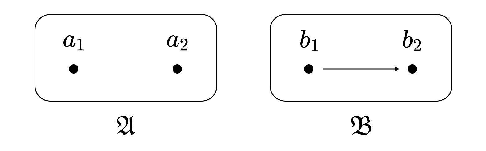
$\mathfrak{A}$의 원소들은 $<^\mathfrak{A}$를 만족시키는 경우가 없으므로 $f: a_1 \mapsto b_1, a_2 \mapsto b_2$는 자명하게 준동형사상이며, 단사이다. 그러나 $f$는 임베딩이 아니다. $f$가 임베딩이라면 $b_1 <^\mathfrak{B} b_2$으로부터 $a_1 <^\mathfrak{A} a_2$가 성립해야 하기 때문이다. 즉, 임베딩은 $\mathfrak{A}$의 원소들뿐 아니라 원소들 간의 관계까지 그대로 $\mathfrak{B}$에 대응시켜야 한다. 이런 면에서 임베딩은 범주론에서의 포화된 함자_{full functor}와 비슷하다.

정의. $\mathfrak{A}$가 언어 $\mathcal{L}$의 구조라고 하자. $\mathcal{L}_\mathfrak{A}$를 $\mathcal{L}$에 $\mathfrak{A}$의 정의역 크기만큼의 상수를 추가한 언어로 정의한다.

페아노 산술로 예를 들자면, $\mathcal{L} = (0, S, +)$이고 $\mathfrak{A}$가 산술의 표준 모형일 때, $\mathcal{L}_\mathfrak{A} = (0, 1, 2, 3, \dots, S, +)$이다.

정의. $\mathfrak{A}$가 만족시키는 모든 $\mathcal{L}_\mathfrak{A}$-원자명제들의 집합을 $\Delta_\mathfrak{A}^+$로 적는다. 즉,

\[\Delta_\mathfrak{A}^+ = \{ R(c_1, \dots, c_n) \mid R, c_i \in \mathcal{L}_\mathfrak{A}, \; \mathfrak{A} \vDash R^{\mathfrak{A}}(c_1^\mathfrak{A}, \dots, c_n^\mathfrak{A}) \}\]

추가로, $\Delta_\mathfrak{A}^+$에다 $\mathfrak{A}$가 만족시키지 않는 모든 $\mathcal{L}$-원자명제들의 부정까지 추가한 집합을 $\Delta_\mathfrak{A}$로 적는다. 즉,

\[\Delta_\mathfrak{A} = \Delta_\mathfrak{A}^+ \cup \{ \lnot R(c_1, \dots, c_n) \mid R, c_i \in \mathcal{L}_\mathfrak{A}, \; \mathfrak{A} \not\vDash R^{\mathfrak{A}}(c_1^\mathfrak{A}, \dots, c_n^\mathfrak{A}) \}\]

$\Delta$라는 표기법은 산술 위계와 관련이 있다.

$\Delta_\mathfrak{A}^+$에 빠진 원자명제들의 부정을 추가한 것이 곧 $\Delta_\mathfrak{A}$이기 때문에, 두 집합이 내포하는 정보량은 사실상 같다. 그럼에도 두 집합을 구분하여 정의하는 것은 다음의 정리 때문이다.

정리. $\mathfrak{A}, \mathfrak{B}$가 $\mathcal{L}$-구조라고 하자.

1. 단사 준동형사상 $f: \mathfrak{A} \to \mathfrak{B}$가 존재할 필요충분조건은 $\mathfrak{B}$가 $\Delta_\mathfrak{A}^+$의 $\mathcal{L}_\mathfrak{A}$-모델인 것이다.
2. 임베딩 $f: \mathfrak{A} \to \mathfrak{B}$가 존재할 필요충분조건은 $\mathfrak{B}$가 $\Delta_\mathfrak{A}$의 $\mathcal{L}_\mathfrak{A}$-모델인 것이다.

즉, $\mathfrak{B}$가 $\Delta_\mathfrak{A}^+$를 만족할 경우 $\mathfrak{B}$가 원자명제들을 ‘과도하게’ 만족시켜서, $\mathfrak{A}$가 $\mathfrak{B}$로 임베딩되지 못할 가능성이 있다. 그러나 $\mathfrak{B}$가 $\Delta_\mathfrak{A}$를 만족할 경우, $\mathfrak{B}$가 만족시킬 수 있는 원자명제에 한계가 걸리기 때문에 임베딩 가능성이 보장된다.

이전 글에서 초등적 부분모델이라는 개념을 소개한 바 있다. 이로부터 다음의 개념을 정의할 수 있다.

정의. $f: \mathfrak{A} \to \mathfrak{B}$가 임베딩이고, $f[\mathfrak{A}]$가 $\mathfrak{B}$의 초등적 부분모델일 때, $f$를 초등적 임베딩이라고 한다.

초등적 임베딩과 관련된 문장 집합은 다음과 같다.

정의. $\mathfrak{A}$가 만족시키는 모든 $\mathcal{L}_\mathfrak{A}$-명제들의 집합을 $E(\mathfrak{A})$로 적는다. 즉,

\[E(\mathfrak{A}) = \{ \phi : \mathfrak{A} \vDash \phi \}\]

$E(\mathfrak{A})$가 $\Delta_\mathfrak{A}$와 가장 구별되는 특징은 양화사가 있는 문장 또한 포함한다는 것이다.

정리. $\mathfrak{A}, \mathfrak{B}$가 $\mathcal{L}$-구조라고 하자. 초등적 임베딩 $f: \mathfrak{A} \to \mathfrak{B}$가 존재할 필요충분조건은 $\mathfrak{B}$가 $E(\mathfrak{A})$의 $\mathcal{L}_\mathfrak{A}$-모델인 것이다.

마지막으로 다음의 문장 집합을 언급할 만하다.

정의. $\mathfrak{A}$가 $\mathcal{L}$-구조라고 하자. $\mathfrak{A}$에서 참인 모든 $\mathcal{L}$-문장들의 집합을 $\mathrm{Th}(\mathfrak{A})$라고 한다.

정리. $\mathfrak{A}, \mathfrak{B}$가 $\mathcal{L}$-구조라고 하자. $\mathfrak{A}$와 $\mathfrak{B}$가 초등적으로 동등할 필요충분조건은 $\mathrm{Th}(\mathfrak{A}) = \mathrm{Th}(\mathfrak{B})$인 것이다.

사실 이는 초등적 동등성의 정의나 다름이 없어서 정리라고 부르기는 무색하지만, 이 글에서 소개한 나머지 정리들과 일관성을 유지하기 위해 소개하였다.

표로 정리하면 이렇다.

	정의	예시	사상
$\Delta_\mathfrak{A}^+$	$\mathfrak{A}$가 만족시키는 $\mathcal{L}_\mathfrak{A}$-원자명제	$0 < 1$	전사 준동형
$\Delta_\mathfrak{A}$	$\mathfrak{A}$가 만족시키는 $\Delta_0$ $\mathcal{L}_\mathfrak{A}$-명제	$\lnot(1 < 0)$	임베딩 (부분모델)
$\mathrm{Th}(\mathfrak{A})$	$\mathfrak{A}$가 만족시키는 $\mathcal{L}$-명제	$\forall x \exists y (x < y)$	초등적 동등성
$E(\mathfrak{A})$	$\mathfrak{A}$가 만족시키는 $\mathcal{L}_\mathfrak{A}$-명제	$\not \exists x (x < 0)$	초등적 임베딩 (초등적 부분모델)

예를 들어 $\mathfrak{A} = (\mathbb{N}, <)$은 $\mathfrak{B} = (\mathbb{Z}, <)$에 임베딩되지만, 초등적으로 임베딩되지는 않는다. $\mathfrak{B}$가 $E(\mathfrak{A})$의 문장인 $\not \exists x (x < 0)$을 만족하지 않기 때문이다.