디멘의 블로그 Jeongdam's Blog
Homomorphisms, Embeddings, and Elementary Embeddings
01 May 2025This post was originally written in Korean, and has been machine translated into English. It may contain minor errors or unnatural expressions. Proofreading will be done in the near future.
For convenience, this article takes the approach of reducing function expressions $f(a) = c$ to binary predicates $F(a, c)$, rather than treating predicates and functions as separate objects.
Definition. Let $\mathfrak{A}, \mathfrak{B}$ be structures of language $\mathcal{L}$. A mapping $f: \mathfrak{A} \to \mathfrak{B}$ satisfying the following is called a homomorphism. For any relation $R$ in $\mathcal{L}$ and arbitrary $a_1, \dots, a_n \in \mathfrak{A}$,
\[R^\mathfrak{A}(a_1, \dots, a_n) \implies R^\mathfrak{B}(f(a_1), \dots, f(a_n))\]Additionally, when a homomorphism $f$ is injective and satisfies the following, we call $f$ an embedding.
\[R^\mathfrak{A}(a_1, \dots, a_n) \iff R^\mathfrak{B}(f(a_1), \dots, f(a_n))\]
An injective homomorphism is not necessarily an embedding. For example, consider the following two structures of language $\mathcal{L}$ with one binary relation $<$. Objects satisfying $<$ are indicated by arrows. That is, $b_1 <^\mathfrak{B} b_2$.
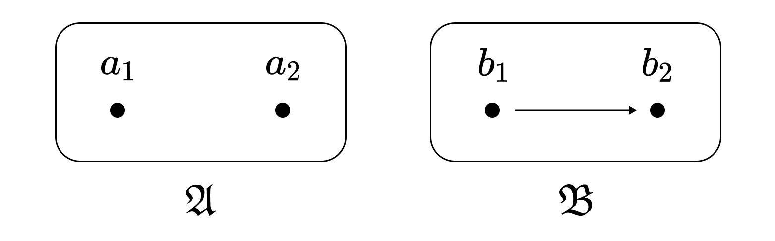
Since no elements in $\mathfrak{A}$ satisfy $<^\mathfrak{A}$, the mapping $f: a_1 \mapsto b_1, a_2 \mapsto b_2$ is trivially a homomorphism and is injective. However, $f$ is not an embedding. If $f$ were an embedding, then from $b_1 <^\mathfrak{B} b_2$ it would follow that $a_1 <^\mathfrak{A} a_2$. That is, an embedding must preserve not only the elements of $\mathfrak{A}$ but also the relationships between elements in $\mathfrak{B}$. In this respect, embeddings are similar to full functors in category theory.
Definition. Let $\mathfrak{A}$ be a structure of language $\mathcal{L}$. Define $\mathcal{L}_\mathfrak{A}$ as the language obtained by adding to $\mathcal{L}$ as many constants as the size of the domain of $\mathfrak{A}$.
For example with Peano arithmetic, when $\mathcal{L} = (0, S, +)$ and $\mathfrak{A}$ is the standard model of arithmetic, then $\mathcal{L}_\mathfrak{A} = (0, 1, 2, 3, \dots, S, +)$.
Definition. Let $\Delta_\mathfrak{A}^+$ denote the set of all $\mathcal{L}_\mathfrak{A}$-atomic propositions satisfied by $\mathfrak{A}$. That is,
\[\Delta_\mathfrak{A}^+ = \{ R(c_1, \dots, c_n) \mid R, c_i \in \mathcal{L}_\mathfrak{A}, \; \mathfrak{A} \vDash R^{\mathfrak{A}}(c_1^\mathfrak{A}, \dots, c_n^\mathfrak{A}) \}\]Additionally, let $\Delta_\mathfrak{A}$ denote the set obtained by adding to $\Delta_\mathfrak{A}^+$ the negations of all $\mathcal{L}$-atomic propositions not satisfied by $\mathfrak{A}$. That is,
\[\Delta_\mathfrak{A} = \Delta_\mathfrak{A}^+ \cup \{ \lnot R(c_1, \dots, c_n) \mid R, c_i \in \mathcal{L}_\mathfrak{A}, \; \mathfrak{A} \not\vDash R^{\mathfrak{A}}(c_1^\mathfrak{A}, \dots, c_n^\mathfrak{A}) \}\]
The notation $\Delta$ is related to the arithmetic hierarchy.
Since $\Delta_\mathfrak{A}$ is obtained by adding the negations of atomic propositions missing from $\Delta_\mathfrak{A}^+$, the two sets contain essentially the same information. Nevertheless, we define the two sets separately because of the following theorem.
Theorem. Let $\mathfrak{A}, \mathfrak{B}$ be $\mathcal{L}$-structures.
- There exists an injective homomorphism $f: \mathfrak{A} \to \mathfrak{B}$ if and only if $\mathfrak{B}$ is an $\mathcal{L}\mathfrak{A}$-model of $\Delta\mathfrak{A}^+$.
- There exists an embedding $f: \mathfrak{A} \to \mathfrak{B}$ if and only if $\mathfrak{B}$ is an $\mathcal{L}\mathfrak{A}$-model of $\Delta\mathfrak{A}$.
That is, when $\mathfrak{B}$ satisfies $\Delta_\mathfrak{A}^+$, there is a possibility that $\mathfrak{B}$ satisfies atomic propositions ‘excessively’, preventing $\mathfrak{A}$ from being embedded into $\mathfrak{B}$. However, when $\mathfrak{B}$ satisfies $\Delta_\mathfrak{A}$, there are constraints on which atomic propositions $\mathfrak{B}$ can satisfy, thus guaranteeing the possibility of embedding.
In a previous article, we introduced the concept of elementary submodel. From this, we can define the following concept.
Definition. When $f: \mathfrak{A} \to \mathfrak{B}$ is an embedding and $f[\mathfrak{A}]$ is an elementary submodel of $\mathfrak{B}$, we call $f$ an elementary embedding.
The set of sentences related to elementary embeddings is as follows.
Definition. Let $E(\mathfrak{A})$ denote the set of all $\mathcal{L}_\mathfrak{A}$-propositions satisfied by $\mathfrak{A}$. That is,
\[E(\mathfrak{A}) = \{ \phi : \mathfrak{A} \vDash \phi \}\]
The most distinguishing feature of $E(\mathfrak{A})$ from $\Delta_\mathfrak{A}$ is that it also includes sentences with quantifiers.
Theorem. Let $\mathfrak{A}, \mathfrak{B}$ be $\mathcal{L}$-structures. There exists an elementary embedding $f: \mathfrak{A} \to \mathfrak{B}$ if and only if $\mathfrak{B}$ is an $\mathcal{L}_\mathfrak{A}$-model of $E(\mathfrak{A})$.
Finally, the following set of sentences is worth mentioning.
Definition. Let $\mathfrak{A}$ be an $\mathcal{L}$-structure. Let $\mathrm{Th}(\mathfrak{A})$ denote the set of all $\mathcal{L}$-sentences true in $\mathfrak{A}$.
Theorem. Let $\mathfrak{A}, \mathfrak{B}$ be $\mathcal{L}$-structures. $\mathfrak{A}$ and $\mathfrak{B}$ are elementarily equivalent if and only if $\mathrm{Th}(\mathfrak{A}) = \mathrm{Th}(\mathfrak{B})$.
In fact, this is nothing more than the definition of elementary equivalence, so it hardly deserves to be called a theorem, but it has been included here to maintain consistency with the other theorems introduced in this article.
Summarising in a table:
| Definition | Example | Mapping | |
|---|---|---|---|
| $\Delta_\mathfrak{A}^+$ | $\mathcal{L}_\mathfrak{A}$-atomic propositions satisfied by $\mathfrak{A}$ | $0 < 1$ | Surjective homomorphism |
| $\Delta_\mathfrak{A}$ | $\Delta_0$ $\mathcal{L}_\mathfrak{A}$-propositions satisfied by $\mathfrak{A}$ | $\lnot(1 < 0)$ | Embedding (submodel) |
| $\mathrm{Th}(\mathfrak{A})$ | $\mathcal{L}$-propositions satisfied by $\mathfrak{A}$ | $\forall x \exists y (x < y)$ | Elementary equivalence |
| $E(\mathfrak{A})$ | $\mathcal{L}_\mathfrak{A}$-propositions satisfied by $\mathfrak{A}$ | $\not \exists x (x < 0)$ | Elementary embedding (elementary submodel) |
For example, $\mathfrak{A} = (\mathbb{N}, <)$ embeds into $\mathfrak{B} = (\mathbb{Z}, <)$, but does not embed elementarily. This is because $\mathfrak{B}$ does not satisfy the sentence $\not \exists x (x < 0)$ from $E(\mathfrak{A})$.
연속체 가설과 동치인 색칠 문제
24 Apr 2025문제. 좌표평면을 가산 개의 색깔을 사용하여 칠했을 때, 세 꼭짓점이 같은 색깔인 직각삼각형이 언제나 존재하는가?
예를 들어 다음의 색칠은 3개의 색깔을 사용하는데, 세 꼭짓점이 모두 같은 색인 직각삼각형을 쉽게 찾을 수 있다.
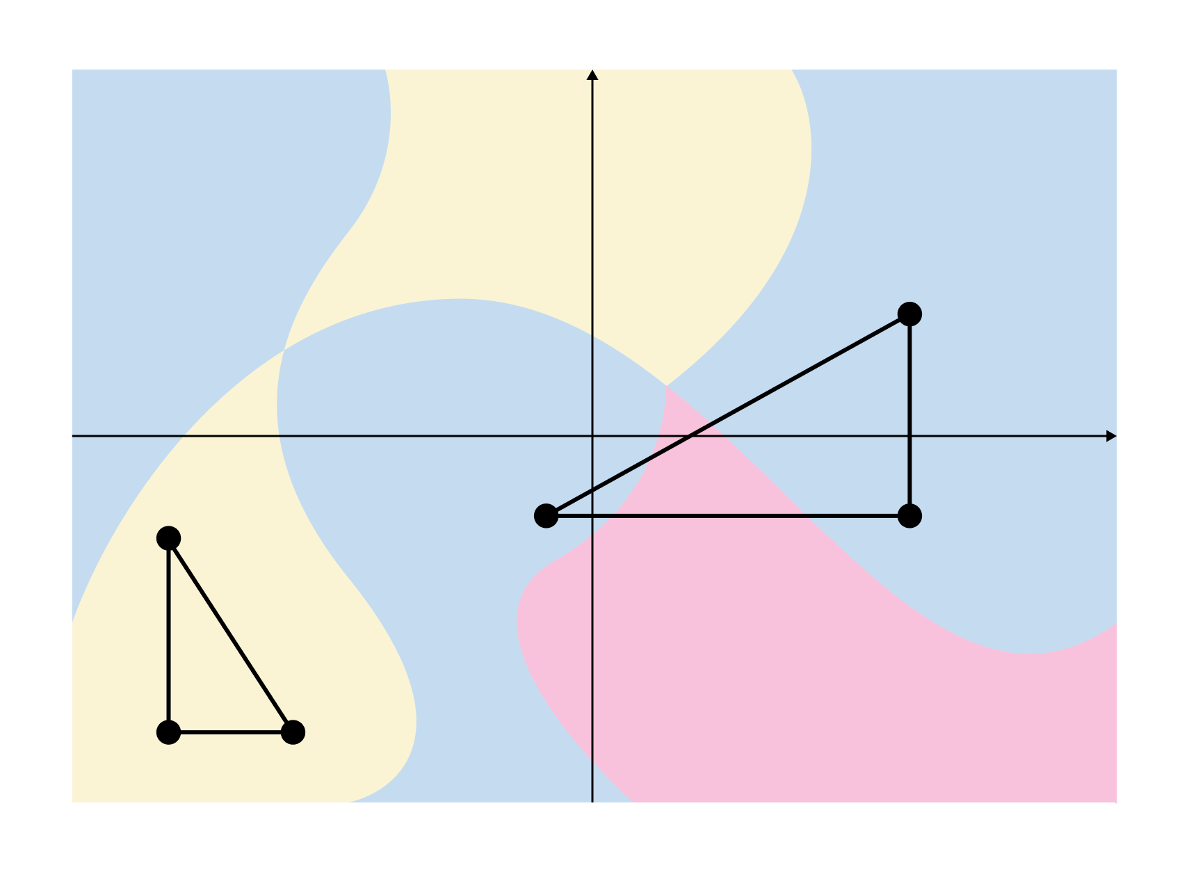
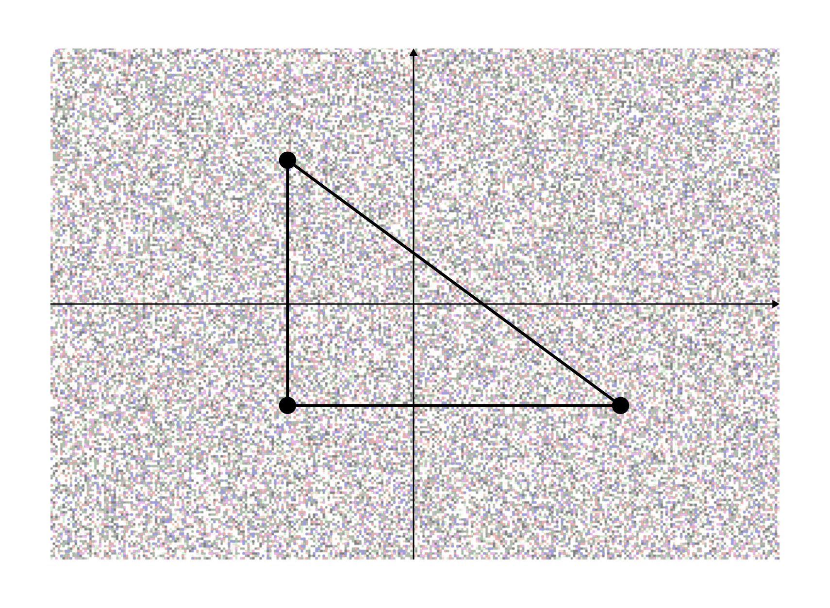
물론 위의 경우는 단순한 경우이고, 아래와 같이 무한히 많은 색깔들이 매우 불규칙적으로 칠해져 있는 경우에도 문제의 직각삼각형이 존재하는지를 따져야 한다.
놀랍게도 언뜻 자명해 보이는 이 문제는 연속체 가설과 동치이다.
연속체 가설. 자연수보다 크고 실수보다 작은 무한집합은 존재하지 않는다.
가장 작은 무한집합인 자연수의 기수를 $\aleph_0$, 자연수보다 큰 무한집합 중 가장 작은 무한집합의 기수를 $\aleph_1$이라고 정의한다. 한편 실수는 자연수의 멱집합과 크기가 같음을 쉽게 보일 수 있으며 집합 $X$의 멱집합은 크기가 $2^{|X|}$이므로, 실수의 기수는 $2^{\aleph_0}$이다. 따라서 연속체 가설의 진술은 $\aleph_1 = 2^{\aleph_0}$와 같다.
정리. 문제의 반례가 존재할 필요충분조건은 $\aleph_1 = 2^{\aleph_0}$이다.
참고로 아래 증명은 필자가 구상한 것이기 때문에 오류가 있을 수도 있다.
증명. $\aleph_1 = 2^{\aleph_0}$라면 문제의 반례가 존재함과, 문제의 반례가 존재하면 $\aleph_1 = 2^{\aleph_0}$임을 각각 보인다.
$\aleph_1 = 2^{\aleph_0}$라면 문제의 반례가 존재한다.
가장 작은 비가산 서수 $\omega_1$에 대해, $\omega_1^2$은 세 꼭짓점이 같은 색인 직각삼각형이 존재하지 않도록 색칠하는 다음의 방법이 존재한다. 먼저 가산 개의 색을 정수와 일대일 대응시킨다. $\alpha < \omega_1$은 가산 서수이므로, 빨간색 선분 $\lbrace (\beta, \alpha) : 0 \leq \beta \leq \alpha \rbrace $의 모든 점을 서로 다른 가산 개의 색으로 칠할 수 있다. 이들 점을 양의 정수에 대응되는 색들로 칠한다. 한편 파란색 선분 $\lbrace (\alpha, \beta) : 0 \leq \beta < \alpha \rbrace $의 점들은 음의 정수에 대응되는 색들로 칠한다.
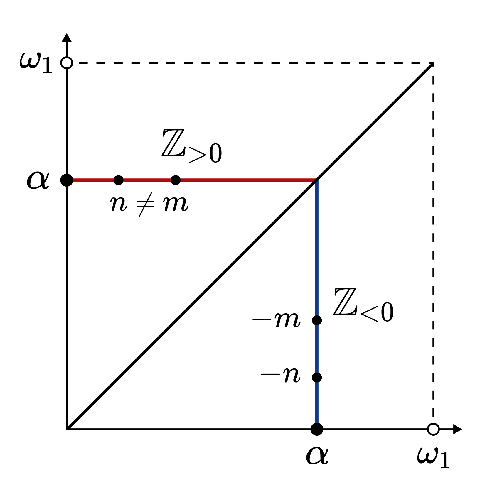
위와 같이 색칠했을 때 세 꼭짓점이 모두 같은 색인 직각삼각형이 없음을 쉽게 보일 수 있다.
만약 $\aleph_1 = 2^{\aleph_0}$라면, 어떤 일대일 대응 $f: \mathbb{R} \to \omega_1$이 존재한다. 이제 평면의 색칠을 다음과 같이 정의한다. 점 $p = (x, y) \in \mathbb{R}^2$을 점 $f(p) = (f(x), f(y)) \in \omega_1^2$와 같은 색으로 칠한다. $f$가 일대일 대응이기 때문에, 만약 해당 색칠해서 점 $p_1, p_2, p_3$가 색깔이 같은 직각삼각형의 세 꼭짓점이라면 $f(p_1), f(p_2), f(p_3)$ 또한 색깔이 같은 직각삼각형의 세 꼭짓점이다. 그런데 그러한 삼각형은 $\omega_1^2$에서 존재하지 않음을 보였으므로, 평면 또한 해당 색칠에서 요구되는 직각삼각형을 가지지 않는다.
문제의 반례가 존재한다면 $\aleph_1 = 2^{\aleph_0}$이다.
$2^{\aleph_0} > \aleph_1$이라고 가정하고 모순을 이끌어 내자. $I$가 크기 $\aleph_1$인 실수의 부분집합이라고 하자. 평면의 부분집합 $X = I \times \mathbb{R}$을 고려하자.
$x$축과 평행인 $X$의 직선들의 집합을 $L_0$라고 하자. $l \in L_0$에 대해, $l$을 이루는 점들 중 색깔 $c$로 칠해진 점의 개수가 $\aleph_1$ 이상일 때, $c \in \aleph_1(l)$이라고 적자. 임의의 $l \in L_0$에 대해, $|l| = \aleph_1$이므로 비둘기집의 원리에 의해 $c \in \aleph_1(l)$인 색깔 $c$가 직선마다 적어도 하나 존재함을 확인하라.
또한 $|L_0| = 2^{\aleph_0}$이므로 비둘기집의 원리에 의해 어떤 색깔 $c_0$가 존재하여, $c_0 \in \aleph_1(l)$을 만족하는 직선 $l$의 개수가 $2^{\aleph_0}$이다. 그러한 직선들의 집합 $L_0’$을 고려하자. $L_0’$의 직선들을 지나는 수직선을 그었을 때 어느 두 교점의 색이 $c_0$라면, 세 꼭짓점의 색이 모두 $c_0$인 직각삼각형이 존재하게 된다. 따라서 임의의 수직선과 $L_0’$의 직선들이 이루는 교점 중 $c_0$로 칠해진 점은 최대 1개이다. 수직선의 개수가 총 $|I| = \aleph_1$개이므로, $L_0’$에는 총 $\aleph_1$개의 $c_0$ 점들이 존재한다.
해당 점들을 모두 빼면 듬성듬성한 직선들의 집합이 된다. 이 집합을 $L_1$이라고 하자.
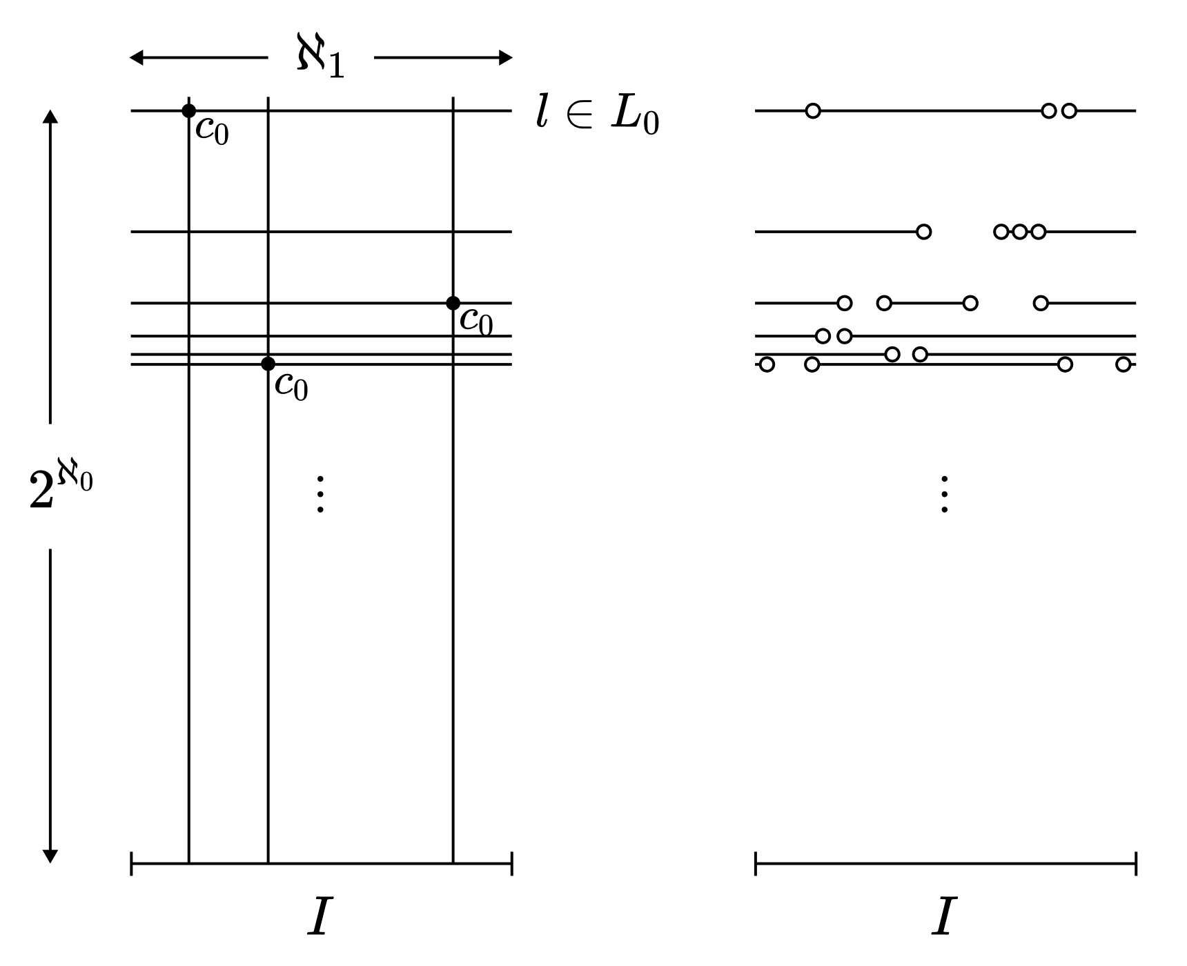
두 가지 경우가 가능하다. a) $L_1$의 직선들 중 $\aleph_1$개의 점들을 가지는 직선이 $2^{\aleph_0}$개이다. b) $L_1$의 직선들 중 $\aleph_1$개의 점들을 가지는 직선이 $\aleph_1$개 이하이다.
a의 경우, 다시 비둘기집의 원리에 의해 $c_1 \in \aleph_1(l)$을 만족하는 직선 $l \in L_1$의 개수가 $2^{\aleph_0}$인 색깔 $c_1$이 존재한다. 그러한 $L_1$의 직선들의 집합을 $L_1’$이라고 하자. 앞선 논의에 의해 $L_1’$에는 총 $\aleph_1$개의 $c_1$ 점들이 존재한다. 이 점들을 뺀 집합을 $L_2$라고 하자. 이같은 과정을 b가 될 때까지 반복한다. (색깔이 가산 개 있기 때문에 언젠가는 b에 도달함을 확인하라)
b가 되었을 때 $L_n$은 최대 $\aleph_1$개의 점들을 가진다. 그런데 $L$이 $L_n$이 되는 과정에서 빠진 점들의 개수는 $\aleph_1 \cdot \aleph_0 = \aleph_1$을 넘지 않는다. 한편 $L$은 $2^{\aleph_0}$개의 점들을 가지고 있었기 때문에, 이는 $\aleph_1 < 2^{\aleph_0}$에 모순된다. ■
A Colouring Problem Equivalent to the Continuum Hypothesis
24 Apr 2025This post was originally written in Korean, and has been machine translated into English. It may contain minor errors or unnatural expressions. Proofreading will be done in the near future.
Problem. When the coordinate plane is coloured using countably many colours, does there always exist a right triangle whose three vertices are of the same colour?
For instance, the following colouring uses 3 colours, and one can easily find a right triangle whose three vertices are all of the same colour.
Of course, the above case is a simple one, and we must consider whether the required right triangle exists even when infinitely many colours are applied in a highly irregular manner, as shown below.
Remarkably, this problem, which appears trivial at first glance, is equivalent to the continuum hypothesis.
Continuum Hypothesis. There exists no infinite set whose cardinality is greater than that of the natural numbers but smaller than that of the real numbers.
We define $\aleph_0$ as the cardinality of the smallest infinite set, namely the natural numbers, and $\aleph_1$ as the cardinality of the smallest infinite set larger than the natural numbers. Meanwhile, the real numbers can easily be shown to have the same cardinality as the power set of the natural numbers, and since the power set of a set $X$ has cardinality $2^{|X|}$, the cardinality of the real numbers is $2^{\aleph_0}$. Therefore, the statement of the continuum hypothesis is equivalent to $\aleph_1 = 2^{\aleph_0}$.
Theorem. A counterexample to the problem exists if and only if $\aleph_1 = 2^{\aleph_0}$.
Note that the following proof is conceived by the author and may contain errors.
Proof. We shall show that if $\aleph_1 = 2^{\aleph_0}$, then a counterexample to the problem exists, and conversely, if a counterexample to the problem exists, then $\aleph_1 = 2^{\aleph_0}$.
If $\aleph_1 = 2^{\aleph_0}$, then a counterexample to the problem exists.
For the smallest uncountable ordinal $\omega_1$, there exists a method of colouring $\omega_1^2$ such that no right triangle with three vertices of the same colour exists. First, we establish a one-to-one correspondence between countably many colours and the integers. Since $\alpha < \omega_1$ is a countable ordinal, we can colour all points of the red segment $\lbrace (\beta, \alpha) : 0 \leq \beta \leq \alpha \rbrace $ with countably many distinct colours. We colour these points with colours corresponding to positive integers. Meanwhile, the points of the blue segment $\lbrace (\alpha, \beta) : 0 \leq \beta < \alpha \rbrace $ are coloured with colours corresponding to negative integers.
It can easily be shown that with this colouring, there exists no right triangle whose three vertices are all of the same colour.
If $\aleph_1 = 2^{\aleph_0}$, then there exists a one-to-one correspondence $f: \mathbb{R} \to \omega_1$. We now define a colouring of the plane as follows. A point $p = (x, y) \in \mathbb{R}^2$ is coloured with the same colour as the point $f(p) = (f(x), f(y)) \in \omega_1^2$. Since $f$ is a one-to-one correspondence, if points $p_1, p_2, p_3$ form the three vertices of a right triangle of the same colour under this colouring, then $f(p_1), f(p_2), f(p_3)$ also form the three vertices of a right triangle of the same colour. However, since we have shown that no such triangle exists in $\omega_1^2$, the plane also lacks the required right triangle under this colouring.
If a counterexample to the problem exists, then $\aleph_1 = 2^{\aleph_0}$.
Suppose $2^{\aleph_0} > \aleph_1$ and derive a contradiction. Let $I$ be a subset of the real numbers with cardinality $\aleph_1$. Consider the subset $X = I \times \mathbb{R}$ of the plane.
Let $L_0$ denote the set of lines in $X$ parallel to the $x$-axis. For $l \in L_0$, we write $c \in \aleph_1(l)$ when the number of points in $l$ coloured with colour $c$ is at least $\aleph_1$. For any $l \in L_0$, since $|l| = \aleph_1$, verify that by the pigeonhole principle, there exists at least one colour $c$ such that $c \in \aleph_1(l)$ for each line.
Moreover, since $|L_0| = 2^{\aleph_0}$, by the pigeonhole principle there exists some colour $c_0$ such that the number of lines $l$ satisfying $c_0 \in \aleph_1(l)$ is $2^{\aleph_0}$. Consider the set $L_0’$ of such lines. When vertical lines are drawn through the lines in $L_0’$, if any two intersection points have colour $c_0$, then there exists a right triangle whose three vertices are all of colour $c_0$. Therefore, amongst the intersection points of any vertical line with the lines in $L_0’$, at most one point is coloured $c_0$. Since there are $|I| = \aleph_1$ vertical lines in total, there exist $\aleph_1$ points of colour $c_0$ in $L_0’$.
Removing all these points yields a sparse set of lines. Let this set be $L_1$.
Two cases are possible: a) There are $2^{\aleph_0}$ lines in $L_1$ that contain $\aleph_1$ points. b) There are at most $\aleph_1$ lines in $L_1$ that contain $\aleph_1$ points.
In case a), again by the pigeonhole principle, there exists a colour $c_1$ such that the number of lines $l \in L_1$ satisfying $c_1 \in \aleph_1(l)$ is $2^{\aleph_0}$. Let $L_1’$ denote the set of such lines in $L_1$. By the previous argument, there exist $\aleph_1$ points of colour $c_1$ in $L_1’$. Let $L_2$ denote the set obtained by removing these points. Repeat this process until case b) is reached. (Verify that case b) is eventually reached since there are countably many colours.)
When case b) is reached, $L_n$ contains at most $\aleph_1$ points. However, the number of points removed in the process from $L$ to $L_n$ does not exceed $\aleph_1 \cdot \aleph_0 = \aleph_1$. Meanwhile, since $L$ originally contained $2^{\aleph_0}$ points, this contradicts $\aleph_1 < 2^{\aleph_0}$. ■
기수의 정의에 관한 노트
20 Apr 2025정의. $X$에서 $Y$로 가는 단사 사상이 존재할 때, $|X| \leq |Y|$라고 적는다. 전단사 사상이 존재할 때, $|X| = |Y|$라고 적는다.
집합론을 처음 공부하는 학생들이 흔히 하는 오해는, 위 정의의 $|\cdot|$과 $\leq$를 복소수에서의 $|\cdot|$과 $\leq$와 유사한 것으로 은연 중에 취급하는 것이다. 요컨대 복소수 $z$에 대해 $|z|$가 실수이고 $\leq$가 실수의 대소 관계이듯이, 집합 $X$에 대해 $|X|$는 집합의 크기 — 이른바 기수cardinality이고, $\leq$는 기수의 대소 관계라고 생각하는 것이다.
그러나 이는 문제의 여지가 많은 접근이다. 왜냐하면 위 정의만으로는 기수라는 수학적 대상을 정의할 수 있다는 보장이 없기 때문이다. 우리가 정의한 것은 이항 관계에 불과하다.
이해를 위한 예시를 들어보자. $A$가 $B$를 좋아할 때, $|A| \leq |B|$라고 적을 수 있을 것이다. 그러나 이렇게 적었다고 해서, $|A|$는 ‘$A$의 호감도’를 의미하며 $\leq$가 호감도의 대소 관계라고 해석한다면 완전히 틀린 것이다. 이와 마찬가지로 $|X| \leq |Y|$는 단사 관계의 유무로 정의되는 이항 관계일 뿐, 이 관계 자체가 기수의 개념을 시사하는 것은 아니다.
특히 ZFC에서는 모든 것이 집합이기 때문에, 만약 기수를 정의하고 싶다면 다음의 사실을 논증해야 한다.
정리 1. 임의의 집합 $X, Y$에 대해, 어떤 집합 $\mathrm{Card}(X), \mathrm{Card}(Y)$가 존재하여, 다음이 성립한다.
- $|X| \leq |Y|$ iff $\mathrm{Card}(X) \subseteq \mathrm{Card}(Y)$
- $|X| = |Y|$ iff $\mathrm{Card}(X) = \mathrm{Card}(Y)$
$\mathrm{Card}(X)$를 $X$의 기수라고 부른다.
즉 ① $\mathrm{Card}(X)$를 정의해야 하고, ② 해당 정의에 대해 위 진술이 성립함을 보여야 한다.
표현의 편의를 위해 $|X| \leq |Y|$와 $|X| = |Y|$를 “$Y$가 $X$보다 작지 않다”, ”$X$와 $Y$의 크기가 같다“라고 부르자. ①부터 살펴 보자면, 크게 네 가지 접근이 가능하다. 짤막하게 알아보자면 이렇다.
-
칸토어의 정의
- 정의: $\mathrm{Card}(X)$를 $X$와 크기가 같은 집합들의 집합으로 정의한다.
- 장점: 정의가 가장 직관적임
- 단점: $\mathrm{Card}(X)$는 사실 집합이 아니라 모임class임
-
스콧의 트릭Scott’s trick
- 정의: $X$와 크기가 같은 집합 중 폰 노이만 위계에서 가장 먼저 등장하는 집합의 랭크가 $V_\alpha$일 때, $\mathrm{Card}(X)$를 $V_\alpha$로 정의한다.
- 장점: 모임의 문제 없이 기수를 정의함
- 단점: 정의가 직관적이지 않고 ad-hoc적인 면모가 있음
-
정렬 원리well-ordering theorem를 사용하여 기수를 정의하기
- 정의: $X$의 정렬에 대응되는 서수ordinal들보다 작지 않은 서수 중 가장 작은 서수를 $\mathrm{Card}(X)$로 정의한다.
- 장점: 정의가 다소 직관적이고, 모임의 문제가 없음
- 단점: 선택 공리 없이는 임의의 집합에 대해 해당 집합의 정렬이 존재함을 보장할 수 없음
-
하르토그스 수Hartogs number를 사용하여 기수를 정의하기
- 정의: $X$의 정렬 가능한 부분집합들에 대응되는 서수들보다 큰 서수 중 가장 작은 서수를 $X$의 하르토그수 수로 정의한다.
- 장점: 정의가 어느 정도 직관적이고, 모임의 문제가 없으며, 선택 공리에 의존적이지 않음
- 단점: 다루기 불편하고 제약이 많음
사실 4를 정의로 채택하는 경우는 없지만, 한 가지 가능성으로서 소개했다. 현대 집합론에서는 2 또는 3을 기수의 정의로 채택한다. 두 경우 모두 정리 1이 성립함을 ZFC에서 보일 수 있다.
흥미로운 것은, 스콧의 트릭을 사용하여 기수를 정의하면 선택 공리가 필요하지는 않지만, 스콧의 트릭으로 정의된 기수가 정리 1을 만족함을 보일 때에는 선택 공리가 필요하다는 사실이다. 왜냐하면 다음이 선택 공리와 동치이기 때문이다.
정리 2. 임의의 집합 $X, Y$에 대해, $|X| \leq |Y|$이거나 $|Y| \leq |X|$이다.
즉, 선택 공리를 사용하지 않더라도 a) 스콧의 트릭을 통해 $\mathrm{Card}(X)$를 정의하거나, b) 단사 사상의 유무를 통해 $|X| \leq |Y|$를 정의할 수 있지만, a)와 b)가 맞물린다는 사실을 보일 때는 선택 공리가 필요하다.
Notes on the Definition of Cardinality
20 Apr 2025This post was originally written in Korean, and has been machine translated into English. It may contain minor errors or unnatural expressions. Proofreading will be done in the near future.
Definition. When there exists an injective mapping from $X$ to $Y$, we write $|X| \leq |Y|$. When there exists a bijective mapping, we write $|X| = |Y|$.
A common misunderstanding amongst students first studying set theory is to implicitly treat the $|\cdot|$ and $\leq$ in the above definition as analogous to $|\cdot|$ and $\leq$ for complex numbers. In other words, just as $|z|$ is a real number for a complex number $z$ and $\leq$ is the ordering relation on real numbers, they think that $|X|$ for a set $X$ is the size of the set—the so-called cardinality—and $\leq$ is the ordering relation on cardinalities.
However, this is a problematic approach. This is because there is no guarantee that we can define cardinality as a mathematical object using only the definition above. What we have defined is merely a binary relation.
Let us consider an example for understanding. When $A$ likes $B$, we might write $|A| \leq |B|$. However, if we interpret this notation to mean that $|A|$ represents ‘$A$’s affection level’ and $\leq$ is the ordering relation on affection levels, this would be completely incorrect. Similarly, $|X| \leq |Y|$ is merely a binary relation defined by the existence of an injective mapping; the relation itself does not suggest the concept of cardinality.
In particular, since everything is a set in ZFC, if we wish to define cardinality, we must prove the following fact.
Theorem 1. For any sets $X, Y$, there exist sets $\mathrm{Card}(X), \mathrm{Card}(Y)$ such that the following holds:
- $|X| \leq |Y|$ iff $\mathrm{Card}(X) \subseteq \mathrm{Card}(Y)$
- $|X| = |Y|$ iff $\mathrm{Card}(X) = \mathrm{Card}(Y)$
We call $\mathrm{Card}(X)$ the cardinality of $X$.
That is, we must ① define $\mathrm{Card}(X)$, and ② show that the above statement holds for this definition.
For convenience of expression, let us refer to $|X| \leq |Y|$ and $|X| = |Y|$ as “$Y$ is not smaller than $X$” and “$X$ and $Y$ have the same size”, respectively. Regarding ①, there are broadly four possible approaches. Let us briefly examine them:
-
Cantor’s definition
- Definition: Define $\mathrm{Card}(X)$ as the collection of all sets having the same size as $X$.
- Advantage: The definition is most intuitive
- Disadvantage: $\mathrm{Card}(X)$ is actually a class, not a set
-
Scott’s trick
- Definition: When the rank of the first set to appear in the von Neumann hierarchy amongst sets having the same size as $X$ is $V_\alpha$, define $\mathrm{Card}(X)$ as $V_\alpha$.
- Advantage: Defines cardinality without the class problem
- Disadvantage: The definition is not intuitive and has ad-hoc aspects
-
Defining cardinality using the well-ordering theorem
- Definition: Define $\mathrm{Card}(X)$ as the smallest ordinal that is not smaller than the ordinals corresponding to well-orderings of $X$.
- Advantage: The definition is somewhat intuitive and avoids the class problem
- Disadvantage: Without the axiom of choice, we cannot guarantee the existence of a well-ordering for arbitrary sets
-
Defining cardinality using Hartogs numbers
- Definition: Define the Hartogs number of $X$ as the smallest ordinal greater than the ordinals corresponding to well-orderable subsets of $X$.
- Advantage: The definition is reasonably intuitive, avoids the class problem, and is not dependent on the axiom of choice
- Disadvantage: Inconvenient to handle and has many limitations
In fact, 4 is never used as a definition, but I’ve listed it for reference purpose. In modern set theory, either 2 or 3 is adopted as the definition of cardinality. In both cases, one can prove that Theorem 1 holds in ZFC.
What is interesting is that while the axiom of choice is not required to define cardinality using Scott’s trick, the axiom of choice is needed to prove that cardinality defined by Scott’s trick satisfies Theorem 1. This is because the following is equivalent to the axiom of choice:
Theorem 2. For any sets $X, Y$, either $|X| \leq |Y|$ or $|Y| \leq |X|$.
That is, even without using the axiom of choice, we can a) define $\mathrm{Card}(X)$ through Scott’s trick, or b) define $|X| \leq |Y|$ through the existence of injective mappings, but the axiom of choice is required to prove that a) and b) mesh together.
무한 죄수 모자 문제
18 Apr 2025아마 여러분은 죄수들이 자신의 모자 색을 맞히는 내용의 퍼즐을 제법 보았을 것이다. 예시는 다음과 같다.
3명의 죄수 A, B, C가 일렬로 서 있다. 간부는 검은 모자 2개와 흰 모자 3개 중 세 개를 골라 각 죄수에게 씌우고는, 만약 어느 한 명이라도 자신의 모자의 색을 맞히면 모두 풀려나지만 틀릴 경우 모두 사형에 처해질 것이라고 말한다. 죄수는 자기 앞에 있는 죄수들의 모자 색은 볼 수 있지만, 자신의 모자 색이나 자기 뒤에 있는 죄수들의 모자 색은 볼 수 없다. 오랜 침묵이 흐른 후, 한 죄수가 자신의 모자 색을 정확히 맞혔다. 문제를 맞힌 죄수는 누구인가?
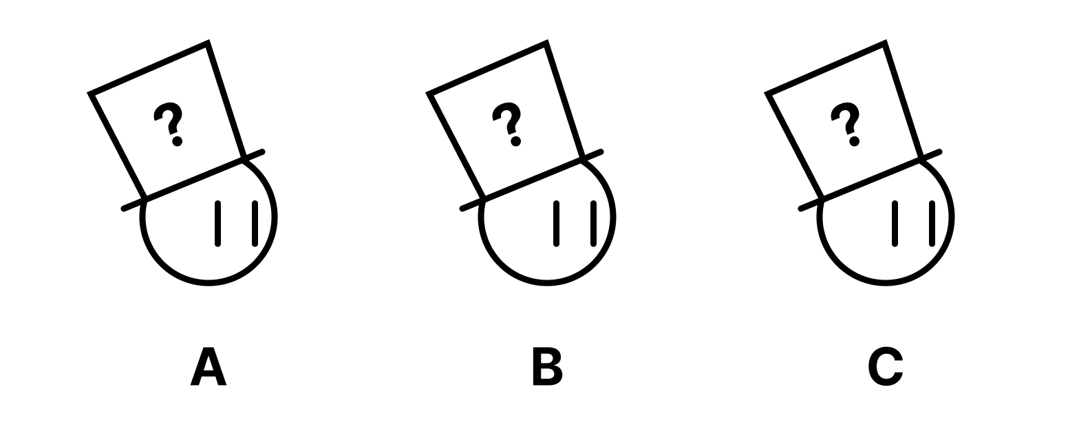
C가 정답을 맞힌다.
만약 B와 C의 모자 색이 모두 검은색이었다면 A는 자신의 모자가 흰색임을 맞혔을 것이다. 그러나 "오랜 침묵"이 흘렀으므로, A는 자신의 모자 색을 맞히지 못하는 상황이며 이는 B, C의 모자 색이 (흰, 검), (검, 흰), (흰, 흰)의 경우 중 하나임을 시사한다.
이 사실을 고려했을 때, 만약 C의 모자 색이 검정색이었다면 B는 자신의 모자 색이 흰색임을 맞혔을 것이다. 그럼에도 "오랜 침묵"이 흘렀다는 것은 B 또한 자신의 모자 색을 맞히지 못하는 상황임을 의미하므로, C의 모자 색은 흰색이다.
조금 더 어려운 문제도 있다.
100명의 죄수가 일렬로 서 있다. 간부는 각 죄수에게 검은 모자와 흰 모자를 무작위로 씌우고는, 1번 죄수부터 차례대로 자신의 모자 색을 맞히게 시킨다. 맞히는 사람은 풀려나지만 틀린 사람은 사형에 처해진다. 죄수들은 사전에 전략을 의논할 수 있지만 모자가 씌워진 이후부터는 정답을 외치는 것 이외의 모든 발언과 행동이 금지된다. 최대 몇 명의 생존을 확실히 보장할 수 있는가?
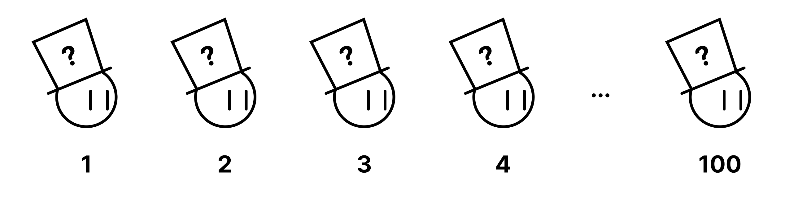
첫 번째 죄수를 제외한 99명의 생존을 보장할 수 있다.
첫 번째 죄수를 제외한 99명의 생존을 보장할 수 있다.
첫 번째 죄수는 자신을 제외한 99명의 모자 색을 볼 수 있다. 그 중 검은색 모자가 짝수 개라면 자신의 모자 색을 검은색으로 맞히고, 홀수 개라면 흰색으로 맞힌다. 그러면 두 번째 죄수는 첫 번째 죄수가 전달한 정보와, 자기 앞에 있는 모자들 중 검은색 모자의 홀짝성을 비교함으로서 자신의 모자 색을 정확히 맞힐 수 있다. 세 번째 죄수 또한 첫 번째 죄수가 전달한 정보와, 두 번째 죄수가 자신의 모자 색을 맞혔다는 사실로부터 자신의 모자 색을 정확히 맞힐 수 있고, 이같은 식으로 99명이 모두 풀려날 수 있다.
이제 문제를 더 괴랄하게 만들어 보자.
무한히 많은 죄수가 일렬로 서 있다. 간부는 각 죄수에게 검은 모자와 흰 모자를 무작위로 씌우고는, 1번 죄수부터 차례대로 자신의 모자 색을 맞히게 시킨다. 맞히는 사람은 풀려나지만 틀린 사람은 사형에 처해진다. 죄수들은 사전에 전략을 의논할 수 있지만 모자가 씌워진 이후부터는 정답을 외치는 것 이외의 모든 발언과 행동이 금지된다. 가능한 적은 죄수가 죽도록 하는 전략은 무엇인가? 단, 모든 죄수는 무한한 연산 능력을 가지며, 수학적으로 전지전능하다고 가정한다. 즉, $f$가 수학적으로 존재하는 함수일 때, 죄수들은 $f$의 함숫값을 언제나 계산할 수 있으며, 사전에 전략을 의논할 때 $f$를 사용하자고 합의할 수 있다.
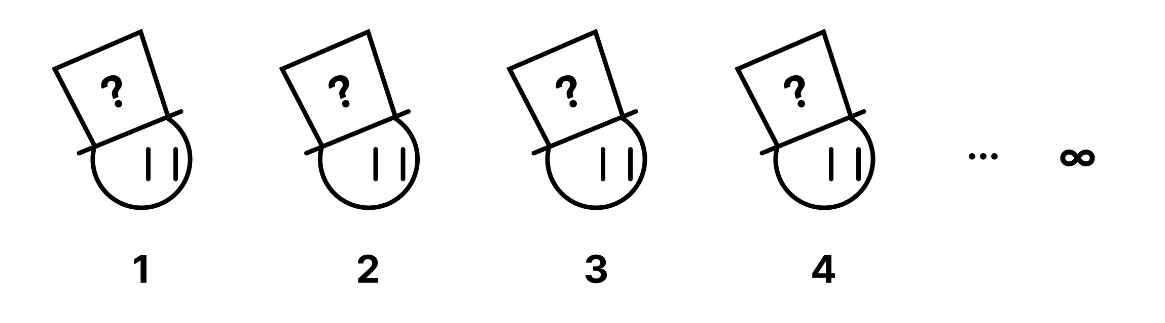
첫 번째 죄수를 제외한 전원의 생존을 보장할 수 있다.
선택 공리를 사용한다.
검은색 모자를 0, 흰색 모자를 1로 적으면 죄수들의 모자 배열은 101011... 와 같은 무한 숫자열로 표현할 수 있다. 앞에 소숫점을 찍고 이진법으로 읽으면 죄수들의 모자 배열은 0 이상 1 이하의 실수와 일대일 대응된다.
실수 $a, b \in [0, 1]$에 대해, $a$와 $b$의 이진 전개가 차이나는 자릿수의 개수가 유한할 때 $a \sim b$라고 하자. 예를 들어,
$$ 0.11111\dots \sim 0.01111\dots, \; 0.10101\dots \not\sim 0.01010\dots $$$\sim$은 동치 관계임을 쉽게 보일 수 있다. 따라서 동치류 $[0, 1]/\sim$을 취할 수 있다. 선택 공리에 의해 $[0, 1]/\sim$의 선택 함수 $\iota$가 존재한다. 죄수들이 수학적으로 전지전능하다고 가정했으므로 사전에 죄수들은 어떤 선택 함수 $\iota$를 사용할지 합의할 수 있다.
모자 맞히기가 시작되었을 때 $n$번째 죄수는 $n$개의 모자를 제외한 모든 모자의 색을 볼 수 있다. 즉, 죄수들의 모자 배열에 대응되는 실수가 $r$일 때, $n$번째 죄수는 $r$의 소숫점 아래 $n$개 자릿수 이외의 모든 자릿수를 알고 있다. 즉, 그는 $r$이 $[0, 1]/\sim$의 어떤 동치류에 속하는지 알며, $r$이 속하는 동치류를 $[r]$이라고 했을 때 $\iota([r])$을 계산할 수 있다.
이제 다음의 전략을 취한다. $\sim$의 정의에 의해 $r$과 $\iota([r])$은 유한한 개수의 자릿수에서만 차이가 난다. 첫 번째 죄수는 자신이 보는 모자들의 배열과 $\iota([r])$에 대응되는 모자들의 배열이 짝수만큼 차이가 나면 자신의 모자색을 검정색으로 맞히고, 홀수만큼 차이가 나면 흰색으로 맞힌다. 이제 나머지 죄수들은 100명의 죄수 문제와 같은 방식으로 자신의 모자 색을 맞힐 수 있다.
즉, 선택 공리는 $N$명의 죄수 문제에서 $N \to \infty$를 취했을 때에도 첫 번째 죄수를 제외한 전원이 생존할 수 있다는 결론이 존속되도록 보장하는 원리이다.
위 퍼즐도 상당히 신기하지만, 다음의 퍼즐은 더 기묘하다.
무한히 많은 죄수가 일렬로 서 있다. 간부는 각 죄수에게 검은 모자와 흰 모자를 무작위로 씌우고는, 1번 죄수부터 차례대로 자신의 모자 색을 맞히게 시킨다. 맞히는 사람은 풀려나지만 틀린 사람은 사형에 처해진다. 죄수들은 사전에 전략을 의논할 수 있지만 모자가 씌워진 이후부터는 정답을 외치는 것 이외의 모든 발언과 행동이 금지된다. 또한, 모자가 씌워지는 순간 죄수들은 청력을 완전히 상실하여 아무런 정보를 주고받을 수 없다. 오직 유한한 수의 죄수만이 죽도록 하는 전략이 있는가? (마찬가지로 죄수는 무한한 연산 능력을 가지며 수학적으로 전지전능하다.)
이전 문제와 같이 $\iota$를 $[0, 1]/\sim$의 선택 함수라고 하자. 다음의 전략을 취한다. $n$번째 죄수는 자신의 모자 색을 $\iota([r])$의 $n$번째 자릿수에 대응되는 색으로 맞힌다. 그러면 $\sim$의 정의에 의해 유한한 수의 죄수를 제외한 전원이 정답을 맞힌다.
위 퍼즐이 특히 기묘한 이유는, 청력 상실 조건에 의해 서로 다른 두 죄수가 모자를 맞히는 사건이 독립이므로, 각각의 죄수가 정답을 맞힐 확률은 $p$로 동일해야 할 듯하기 때문이다. 이 경우 총 $N$명의 죄수가 정답을 맞히는 확률은 $p^N$이 되므로, $N \to \infty$에 따라 확률은 0으로 수렴한다. 그러나 실제로는 무한히 많은 죄수들이 정답을 맞힌다.
이 역설의 뿌리는, 임의의 죄수가 정답을 맞히는 확률이 정의되지 않는다는 데 있다. 잘 생각해 보면, 임의의 죄수가 정답을 맞히는 사건은 주어진 실수 $r \in [0, 1]$이 비탈리 집합에 포함되는 사건과 동일한데, 비탈리 집합은 비가측 집합이므로 이 사건에는 확률을 정의할 수 없기 때문이다.
Infinite Prisoner Hat Problem
18 Apr 2025This post was originally written in Korean, and has been machine translated into English. It may contain minor errors or unnatural expressions. Proofreading will be done in the near future.
You have likely encountered puzzles where prisoners attempt to guess the colour of their own hats. Consider the following example:
Three prisoners A, B, and C stand in a line. A guard selects three hats from two black hats and three white hats, places them on each prisoner, and announces that if any one of them correctly guesses their hat colour, all will be freed, but if they guess incorrectly, all will be executed. Each prisoner can see the hat colours of those in front of them, but cannot see their own hat colour or those of prisoners behind them. After a long silence, one prisoner correctly identifies their hat colour. Which prisoner solved the problem?
C provides the correct answer.
If both B and C wore black hats, A would have correctly guessed that their hat was white. However, since a "long silence" ensued, A could not determine their hat colour, indicating that the hat colours of B and C represent one of the cases: (white, black), (black, white), or (white, white).
Considering this information, if C's hat were black, B would have correctly guessed that their hat was white. The fact that a "long silence" continued indicates that B also could not determine their hat colour, therefore C's hat must be white.
A more challenging problem follows:
One hundred prisoners stand in a line. A guard randomly places either a black or white hat on each prisoner, then instructs them to guess their hat colour in order, starting from prisoner 1. Those who guess correctly are freed, while those who guess incorrectly are executed. The prisoners may discuss strategy beforehand, but after the hats are placed, all communication and actions are forbidden except stating their answer. What is the maximum number of prisoners whose survival can be guaranteed with certainty?
The survival of 99 prisoners, excluding the first, can be guaranteed.
The survival of 99 prisoners, excluding the first, can be guaranteed.
The first prisoner can observe the hat colours of the remaining 99 prisoners. If the number of black hats amongst them is even, they guess their own hat is black; if odd, they guess white. The second prisoner can then compare the information conveyed by the first prisoner with the parity of black hats amongst those in front of them to correctly determine their own hat colour. Similarly, the third prisoner can use the information from the first prisoner and the fact that the second prisoner correctly identified their hat colour to determine their own, and in this manner, all 99 prisoners can be freed.
Let us now make the problem more formidable:
Infinitely many prisoners stand in a line. A guard randomly places either a black or white hat on each prisoner, then instructs them to guess their hat colour in order, starting from prisoner 1. Those who guess correctly are freed, while those who guess incorrectly are executed. The prisoners may discuss strategy beforehand, but after the hats are placed, all communication and actions are forbidden except stating their answer. What strategy minimises the number of prisoners who die? We assume that all prisoners possess infinite computational power and are mathematically omniscient. That is, when $f$ is a mathematically well-defined function, prisoners can always compute the value of $f$, and when discussing strategy beforehand, they may agree to employ $f$.
The survival of all prisoners except the first can be guaranteed.
The axiom of choice is employed.
By representing black hats as 0 and white hats as 1, the prisoners' hat arrangement can be expressed as an infinite sequence such as 101011... When a decimal point is placed at the beginning and read in binary, the prisoners' hat arrangement corresponds bijectively to a real number between 0 and 1 inclusive.
For real numbers $a, b \in [0, 1]$, we define $a \sim b$ when their binary expansions differ in finitely many digits. For example:
$$ 0.11111\dots \sim 0.01111\dots, \; 0.10101\dots \not\sim 0.01010\dots $$It can be readily shown that $\sim$ is an equivalence relation. Therefore, we may form the quotient $[0, 1]/\sim$. By the axiom of choice, there exists a choice function $\iota$ for $[0, 1]/\sim$. Since we have assumed that the prisoners are mathematically omniscient, they can agree beforehand on which choice function $\iota$ to employ.
When the hat-guessing begins, the $n$-th prisoner can observe all hat colours except for $n$ hats. That is, when the real number corresponding to the prisoners' hat arrangement is $r$, the $n$-th prisoner knows all digits except for $n$ digits after the decimal point of $r$. Thus, they know which equivalence class of $[0, 1]/\sim$ contains $r$, and when the equivalence class containing $r$ is denoted $[r]$, they can compute $\iota([r])$.
The following strategy is now employed: By the definition of $\sim$, $r$ and $\iota([r])$ differ in only finitely many digits. The first prisoner guesses their hat colour as black if the hat arrangement they observe differs from the hat arrangement corresponding to $\iota([r])$ by an even number of positions, and white if they differ by an odd number. The remaining prisoners can then determine their hat colours in the same manner as in the 100-prisoner problem.
Thus, the axiom of choice ensures that when taking $N \to \infty$ in the $N$-prisoner problem, the conclusion that all prisoners except the first can survive remains valid.
while the above puzzle is remarkably intriguing, the following puzzle is even more extraordinary:
Infinitely many prisoners stand in a line. A guard randomly places either a black or white hat on each prisoner, then instructs them to guess their hat colour in order, starting from prisoner 1. Those who guess correctly are freed, while those who guess incorrectly are executed. The prisoners may discuss strategy beforehand, but after the hats are placed, all communication and actions are forbidden except stating their answer. Furthermore, the moment the hats are placed, the prisoners completely lose their hearing and cannot exchange any information whatsoever. Is there a strategy that ensures only finitely many prisoners die? (Similarly, prisoners possess infinite computational power and are mathematically omniscient.)
As in the previous problem, let $\iota$ be a choice function for $[0, 1]/\sim$. The following strategy is employed: The $n$-th prisoner guesses their hat colour as the colour corresponding to the $n$-th digit of $\iota([r])$. By the definition of $\sim$, all prisoners except finitely many will answer correctly.
This puzzle is particularly extraordinary because the hearing loss condition renders the hat-guessing events of any two distinct prisoners independent, suggesting that each prisoner should have the same probability $p$ of guessing correctly. In this case, the probability that all $N$ prisoners guess correctly would be $p^N$, which converges to 0 as $N \to \infty$. However, in reality, infinitely many prisoners guess correctly.
The root of this paradox lies in the fact that the probability of an arbitrary prisoner guessing correctly is undefined. Upon careful consideration, the event of an arbitrary prisoner guessing correctly is equivalent to the event that a given real number $r \in [0, 1]$ belongs to a Vitali set. Since Vitali sets are non-measurable, no probability can be defined for this event.
워시-타르스키 보존 정리
17 Apr 2025군 $G$의 부분군 $H, K$에 대해 $H \cap K$는 언제나 군이다. 환과 체의 경우에도 마찬가지이다. 이는 워시-타르스키 정리의 따름결과로 설명할 수 있다.
Notation. 본 글에서 $T$는 언어 $\mathcal{L}$의 1차 논리 이론이며, 프락투르 글자 $\mathfrak{M}, \mathfrak{N}, \dots$은 $\mathcal{L}$-구조structure이다. 또한 $\mathfrak{M}, \mathfrak{N}, \dots$의 정의역을 $M, N, \dots$와 같이 적는다.
기본 개념
정의. $N \subseteq M$이고 $\mathfrak{N}$에서의 해석interpretation이 $\mathfrak{M}$에서의 해석을 $N$으로 제한한 것일 때, $\mathfrak{N}$을 $\mathfrak{M}$의 부분모델submodel이라고 하며, 기호로 $\mathfrak{N} \subseteq \mathfrak{M}$과 같이 적는다. 또한, $\mathfrak{M}$을 $\mathfrak{N}$의 확장extension이라고 한다.
일례로 $(2\mathbb{Z}, +)$는 $(\mathbb{Z}, +)$의 부분모델이고, $(\mathbb{Q}, +, \cdot)$는 $(\mathbb{R}, +, \cdot)$의 부분모델이다.
정의. 임의의 $\mathcal{L}$-문장 $\phi$에 대해 $\mathfrak{M} \vDash \phi \iff \mathfrak{N} \vDash \phi$일 때 $\mathfrak{M}$과 $\mathfrak{N}$이 초등적으로 동등elementarily equivalent하다고 하며, 기호로 $\mathfrak{M} \equiv \mathfrak{N}$과 같이 적는다.
뢰벤하임-스콜렘 정리에 의해 $\kappa$가 $|\mathcal{L}|$ 이상의 무한 기수라면, 임의의 무한 구조 $\mathfrak{M}$과 초등적으로 동등하며 크기가 $\kappa$인 모델 $\mathfrak{N}$이 존재한다. (cf. 워시-보트 판별Łoś-Vaught test)
정의. $\mathfrak{M}$과 $\mathfrak{N}$이 구조적으로 동일할 때 동형isomorphic이라고 하며, 기호로 $\mathfrak{M} \cong \mathfrak{N}$과 같이 적는다. 구체적으로, 어떤 일대일 대응 $\phi: M \to N$이 존재하여, $\mathcal{L}$의 임의의 함수 $f$와 관계 $R$에 대해 다음이 임의의 $a_1, \dots, a_n \in M$에 대해 성립할 때 $\mathfrak{M} \cong \mathfrak{N}$이다.
\[\begin{gather} \phi(f_\mathfrak{M}(a_1, \dots, a_n)) = f_\mathfrak{N}(\phi(a_1), \dots, \phi(a_n)), \\\\ R_\mathfrak{M}(a_1, \dots, a_n) \iff R_\mathfrak{N}(\phi(a_1), \dots, \phi(a_n)) \end{gather}\]
$(\mathbb{Z}, +)$와 $(2\mathbb{Z}, +)$는 $\phi: x \mapsto 2x$를 통해 동형이지만 $(\mathbb{Q}, +, \cdot)$와 $(\mathbb{R}, +, \cdot)$은 동형이 아니다.
다음 정리의 증명은 거의 자명하다.
정리. 동형인 두 구조는 초등적으로 동등하다.
정의. $\mathfrak{N} \subseteq \mathfrak{M}$이라고 하자. 임의의 $\mathcal{L}$-명제 $\phi$와 $\mathfrak{N}$에서의 자유변수 할당assignment $g$에 대해, $\mathfrak{N} \vDash \phi[g] \iff \mathfrak{M} \vDash \phi[g]$일 때 $\mathfrak{N}$이 $\mathfrak{M}$의 초등적 부분모델elementary submodel이라고 하며, 기호로 $\mathfrak{N} \preceq \mathfrak{M}$과 같이 적는다.
2와 3은 1보다 강하지만, 2와 3은 서로를 시사하지 않는다.
- $\mathfrak{N} \subseteq \mathfrak{M}$, $\mathfrak{N} \equiv \mathfrak{M}$
- $\mathfrak{N} \subseteq \mathfrak{M}$, $\mathfrak{N} \cong \mathfrak{M}$
- $\mathfrak{N} \preceq \mathfrak{M}$
2와 3이 서로를 시사하지 않는 이유는, 2가 구조적 동등을 요구한다는 점에서 3보다 약하지 않은 한편, 3이 임의의 할당에 대한 동등을 요구한다는 점에서 2보다 약하지 않기 때문이다. 예를 들어 $\mathfrak{M} = (\mathbb{R}, +, \cdot)$에 대해, $\mathfrak{N}$이 $\mathfrak{M}$의 동형인 부분모델이기 위해서는 구성 가능한 실수에 대해 구조적으로 동일해야 하는 반면, $\mathfrak{N}$이 $\mathfrak{M}$의 초등적 부분모델이기 위해서는 두 모델이 모든 실수에 대해 초등적으로 동등해야 한다.
| 2 | 3 | |
|---|---|---|
| 2가 3보다 약하지 않다 | 구조적 동일성 | 초등적 동일성 |
| 3이 2보다 약하지 않다 | 구성 가능한 대상 | 임의의 대상 |
일례로 앞서 보았듯이 $(2\mathbb{Z}, +)$는 $(\mathbb{Z}, +)$의 동형인 부분모델이지만, $\exists y \; (y + y = x)$에 $x \mapsto 2$ 할당을 고려하면 초등적 부분모델은 아님을 알 수 있다.
워시-타르스키 정리
$\mathfrak{M}$이 $T$의 모델이라고 하자. $T$가 어떤 이론이어야 $\mathfrak{M}$의 임의의 부분모델 또한 $T$의 모델이 될까? 그 답은 다음의 정리로 주어진다.
워시-타르스키Łoś-Tarski 보존 정리. $T$의 모델의 부분모델 또한 $T$의 모델일 필요충분조건은 $T$가 $\Pi_1$ 문장으로 이루어진 이론과 동치인 것이다.
$\Pi_1$ 문장이 무엇인지에 대해서는 산술 위계 글에서 다룬 바 있다. 간략히만 설명하자면 $\forall$만을 양화사로 가지는 이론이다. 직관적으로 $\Pi_1$ 문장은 정의역이 제한될수록 만족시키기 쉬우므로, $T$가 $\Pi_1$ 이론이라면 $T$는 부분모델에 대해 보존될 것이다. 필요조건은 증명하기가 좀 더 까다롭다.
증명. 충분조건은 거의 자명하므로 필요조건만 증명한다. 다음의 보조정리를 증명한다.
보조정리. $T$가 언어 $\mathcal{L}$의 무모순적인 이론이라고 하자. $\mathcal{L}$ 문장들의 집합 $\Delta$가 다음 두 조건을 만족할 때, $\Delta$는 $T$의 공리화를 포함한다.
- $\Delta$는 선언disjunction에 대해 닫혀 있다. 즉, $\phi, \psi \in \Delta$라면 $\phi \lor \psi \in \Delta$이다.
- $T$의 모델 $\mathfrak{A}$에 대해, $\mathfrak{B}$가 $\mathfrak{A}$에서 만족되는 모든 $\Delta$의 문장들을 만족한다면 $\mathfrak{B}$ 또한 $T$의 모델이다.
보조정리의 증명. $\Gamma = \lbrace \delta \in \Delta : T \vDash \delta \rbrace $라고 하자. $\Delta$가 $T$의 공리화를 포함함을 보이기 위해서는 다음을 보이면 충분하다.
\[\mathfrak{B} \vDash \Gamma \implies \mathfrak{B} \vDash T\]$\mathfrak{B}$가 $\Gamma$의 모델이라고 하자. 다음과 같이 정의한다.
\[\Sigma = \{ \lnot \delta : \delta \in \Delta, \mathfrak{B} \not\vDash \delta \}\]$T \cup \Sigma$는 무모순적인 이론임을 보이자. 만약 $T \cup \Sigma$가 모순적이라면 어떤 $\lnot\delta_1, \dots, \lnot\delta_n \in \Sigma$에 대해 $T \vdash \lnot(\lnot\delta_1 \land \cdots \land \lnot\delta_n)$이므로, $T \vdash \delta_1 \lor \cdots \lor \delta_n$이다. $\Delta$가 선언에 대해 닫혀 있으므로 $\delta_1 \lor \cdots \lor \delta_n \in \Delta$이다. $\Gamma$의 정의에 의해 $\delta_1 \lor \cdots \lor \delta_n \in \Gamma$이므로 $\mathfrak{B} \vDash \delta_1 \lor \cdots \lor \delta_n$이다. 이는 $\lnot\delta_1, \dots, \lnot\delta_n \in \Sigma$에 모순이다.
$T \cup \Sigma$가 무모순적이므로 완전성 정리에 의해 모델을 가진다. 해당 모델을 $\mathfrak{A}$라고 하자. $\mathfrak{B}$는 $\mathfrak{A}$가 만족시키는 $\Delta$의 문장들을 모두 만족시키므로, 가정에 의해 $T$의 모델이다. □
이제 본 정리의 증명으로 넘어가자. $\Delta$를 모든 $\mathcal{L}$의 $\Pi_1$ 문장들의 집합이라고 하자. 우리의 목표는 $\Delta$가 $T$의 공리화를 포함함을 보이는 것이다. $\Pi_1$ 문장들은 선언에 대해 닫혀 있으므로, 보조정리에 의해 다음을 보이면 충분하다.
$T$가 부분모델에 대해 보존적인 이론이라고 하자. $T$의 모델 $\mathfrak{A}$에 대해, $\mathfrak{B}$가 $\mathfrak{A}$에서 만족되는 모든 $\Pi_1$ 문장들을 만족한다면 $\mathfrak{B}$ 또한 $T$의 모델이다.
이 글에서의 표기법을 따라 $E(\mathfrak{B})$를 정의하자. 즉, $\mathfrak{M}$이 $E(\mathfrak{B})$를 만족할 때 $\mathfrak{B} \preceq \mathfrak{M}$이다.
$T \cup E(\mathfrak{B})$는 무모순적임을 보이자. 만약 $T \cup E(\mathfrak{B})$가 모순적이라면, 어떤 $E(\mathfrak{B})$의 문장 $\phi(b_1, \dots, b_n)$이 존재하여 $T \cup \lbrace \phi \rbrace $는 모델을 가지지 않는다. 따라서 $T$의 모델인 $\mathfrak{A}$는 $\phi$를 만족시키는 $\mathcal{L} \cup \lbrace b_1, \dots, b_n \rbrace $ 모델로 확장될 수 없다. 즉, 다음이 성립한다.
\[\mathfrak{A} \vDash \forall x_1 \cdots \forall x_n \lnot \phi(x_1, \dots, x_n)\]우변은 $\Pi_1$ 문장이므로, 가정에 의해 $\mathfrak{B} \vDash \forall x_1 \cdots \forall x_n \lnot \phi(x_1, \dots, x_n)$이다. 그런데 $\phi(b_1, \dots, b_n) \in E(\mathfrak{B})$이므로, 이는 모순이다. 따라서 $T \cup E(\mathfrak{B})$는 무모순적이며, 완전성 정리에 의해 모델 $\mathfrak{C}$를 가진다. 그리고 $\mathfrak{C}$는 $E(\mathfrak{B})$를 만족하므로, $\mathfrak{B} \preceq \mathfrak{C}$이다. 한편 $\mathfrak{C}$는 부분모델에 대해 보존적인 이론 $T$의 모델이므로, $\mathfrak{B}$는 $T$의 모델이다. ■
응용
군의 1차 논리적 공리화는, 항등원과 역원을 별도의 상수 $e$와 함수 $(-)^{-1}$로 표현하는지의 여부에 따라 구분된다.
표현하지 않는 경우
언어 $\mathcal{L}_1 = \lbrace G, \cdot \rbrace $의 이론 $T_1$를 다음과 같이 정의한다.
- $\forall x, y, z : (x \cdot y) \cdot z = x \cdot (y \cdot z)$
- $\exists x \forall y : x \cdot y = y \cdot x = y$
- $\forall x \exists y \forall z : (x \cdot y) \cdot z = (y \cdot x) \cdot z = z$
표현하는 경우
언어 $\mathcal{L}_2 = \lbrace G, \cdot, e, (-)^{-1} \rbrace $의 이론 $T_2$를 다음과 같이 정의한다.
- $\forall x, y, z : (x \cdot y) \cdot z = x \cdot (y \cdot z)$
- $\forall x : x \cdot e = e \cdot x = x$
- $\forall x : x \cdot x^{-1} = x^{-1} \cdot x = e$
$T_1$은 $\Pi_1$ 이론이 아니지만 $T_2$는 $\Pi_1$ 이론이다. 따라서 워시-타르스키 정리에 의해, $T_1$은 부분모델 보존적이지 않지만 $T_2$는 보존적이다. $T_1$이 부분모델 보존적이지 않다는 것은, 군의 부분집합이 연산에 대해 닫혀 있다고 해서 언제나 부분군인 것은 아님을 의미한다(일례로 $\mathbb{Z}$의 부분집합 $\mathbb{Z}_{> 0}$은 연산에 대해 닫혀 있지만 역원을 결여하므로 군이 아니다). 반면 $T_2$가 부분모델 보존적이라는 것은 다음이 성립함을 의미한다.
군 $G$에 대해, $G$의 부분집합 $H$가 다음을 만족한다면 $H$는 $G$의 부분군이다.
- 연산에 대해 닫혀 있다.
- 역원에 대해 닫혀 있다.
- $G$의 항등원을 포함한다.
그런데 위보다 더 강한 다음의 결과가 일반적으로 성립한다.
군 $G$에 대해, $G$의 부분집합 $H$가 다음을 만족한다면 $H$는 $G$의 부분군이다.
- 연산에 대해 닫혀 있다.
- 역원에 대해 닫혀 있다.
즉, 항등원을 지시할 상수를 결여하는 언어 $\mathcal{L}_3 = \lbrace G, \cdot, (-)^{-1} \rbrace$에서도 군의 이론은 부분모델 보존적이며, 이는 $\mathcal{L}_3$로 군을 형식화하는 $\Pi_1$ 이론이 존재함을 의미한다. 머리를 잘 굴려보면 실제로 다음의 이론 $T_3$가 존재함을 발견할 수 있다.
- $\forall x, y, z : (x \cdot y) \cdot z = x \cdot (y \cdot z)$
- $\forall x, y : (x \cdot x^{-1}) \cdot y = y \cdot (x \cdot x^{-1}) = y$
The Łoś-Tarski Preservation Theorem
17 Apr 2025This post was originally written in Korean, and has been machine translated into English. It may contain minor errors or unnatural expressions. Proofreading will be done in the near future.
For subgroups $H, K$ of a group $G$, the intersection $H \cap K$ is always a group. The same holds for rings and fields. This can be explained as a consequence of the Łoś-Tarski theorem.
Notation. In this article, $T$ is a first-order theory in language $\mathcal{L}$, and Fraktur letters $\mathfrak{M}, \mathfrak{N}, \dots$ denote $\mathcal{L}$-structures. Furthermore, we write the domains of $\mathfrak{M}, \mathfrak{N}, \dots$ as $M, N, \dots$ respectively.
Basic Concepts
Definition. When $N \subseteq M$ and the interpretation in $\mathfrak{N}$ is the restriction of the interpretation in $\mathfrak{M}$ to $N$, we call $\mathfrak{N}$ a submodel of $\mathfrak{M}$, and write $\mathfrak{N} \subseteq \mathfrak{M}$. Furthermore, $\mathfrak{M}$ is called an extension of $\mathfrak{N}$.
For example, $(2\mathbb{Z}, +)$ is a submodel of $(\mathbb{Z}, +)$, and $(\mathbb{Q}, +, \cdot)$ is a submodel of $(\mathbb{R}, +, \cdot)$.
Definition. When $\mathfrak{M} \vDash \phi \iff \mathfrak{N} \vDash \phi$ for any $\mathcal{L}$-sentence $\phi$, we say that $\mathfrak{M}$ and $\mathfrak{N}$ are elementarily equivalent, and write $\mathfrak{M} \equiv \mathfrak{N}$.
By the Löwenheim-Skolem theorem, if $\kappa$ is an infinite cardinal at least $|\mathcal{L}|$, then for any infinite structure $\mathfrak{M}$, there exists a model $\mathfrak{N}$ of cardinality $\kappa$ that is elementarily equivalent to $\mathfrak{M}$. (cf. Łoś-Vaught test)
Definition. When $\mathfrak{M}$ and $\mathfrak{N}$ are structurally identical, they are called isomorphic, written $\mathfrak{M} \cong \mathfrak{N}$. Specifically, $\mathfrak{M} \cong \mathfrak{N}$ when there exists a bijection $\phi: M \to N$ such that for any function $f$ and relation $R$ in $\mathcal{L}$, the following holds for any $a_1, \dots, a_n \in M$:
\[\begin{gather} \phi(f_\mathfrak{M}(a_1, \dots, a_n)) = f_\mathfrak{N}(\phi(a_1), \dots, \phi(a_n)), \\\\ R_\mathfrak{M}(a_1, \dots, a_n) \iff R_\mathfrak{N}(\phi(a_1), \dots, \phi(a_n)) \end{gather}\]
$(\mathbb{Z}, +)$ and $(2\mathbb{Z}, +)$ are isomorphic via $\phi: x \mapsto 2x$, but $(\mathbb{Q}, +, \cdot)$ and $(\mathbb{R}, +, \cdot)$ are not isomorphic.
The proof of the following theorem is almost trivial.
Theorem. Two isomorphic structures are elementarily equivalent.
Definition. Let $\mathfrak{N} \subseteq \mathfrak{M}$. When $\mathfrak{N} \vDash \phi[g] \iff \mathfrak{M} \vDash \phi[g]$ for any $\mathcal{L}$-formula $\phi$ and any assignment $g$ of free variables in $\mathfrak{N}$, we call $\mathfrak{N}$ an elementary submodel of $\mathfrak{M}$, and write $\mathfrak{N} \preceq \mathfrak{M}$.
Conditions 2 and 3 are stronger than 1, but 2 and 3 do not imply each other.
- $\mathfrak{N} \subseteq \mathfrak{M}$, $\mathfrak{N} \equiv \mathfrak{M}$
- $\mathfrak{N} \subseteq \mathfrak{M}$, $\mathfrak{N} \cong \mathfrak{M}$
- $\mathfrak{N} \preceq \mathfrak{M}$
The reason why 2 and 3 do not imply each other is that 2 requires structural equivalence, making it no weaker than 3, while 3 requires equivalence for arbitrary assignments, making it no weaker than 2. For instance, for $\mathfrak{M} = (\mathbb{R}, +, \cdot)$, for $\mathfrak{N}$ to be an isomorphic submodel of $\mathfrak{M}$, it must be structurally identical with respect to constructible real numbers, whereas for $\mathfrak{N}$ to be an elementary submodel of $\mathfrak{M}$, the two models must be elementarily equivalent with respect to all real numbers.
| 2 | 3 | |
|---|---|---|
| 2 is no weaker than 3 | Structural identity | Elementary identity |
| 3 is no weaker than 2 | Constructible objects | Arbitrary objects |
For example, as we saw earlier, $(2\mathbb{Z}, +)$ is an isomorphic submodel of $(\mathbb{Z}, +)$, but considering the assignment $x \mapsto 2$ for $\exists y \; (y + y = x)$, we can see that it is not an elementary submodel.
The Łoś-Tarski Theorem
Let $\mathfrak{M}$ be a model of $T$. What kind of theory must $T$ be for any submodel of $\mathfrak{M}$ to also be a model of $T$? The answer is given by the following theorem.
The Łoś-Tarski Preservation Theorem. A necessary and sufficient condition for submodels of models of $T$ to also be models of $T$ is that $T$ is equivalent to a theory consisting of $\Pi_1$ sentences.
What $\Pi_1$ sentences are has been covered in the arithmetic hierarchy article. To explain briefly, these are theories having only $\forall$ as quantifiers. Intuitively, $\Pi_1$ sentences become easier to satisfy as the domain is restricted, so if $T$ is a $\Pi_1$ theory, then $T$ will be preserved under submodels. The necessity is somewhat more challenging to prove.
Proof. The sufficiency is almost trivial, so we prove only the necessity. We prove the following lemma.
Lemma. Let $T$ be a consistent theory in language $\mathcal{L}$. When a set $\Delta$ of $\mathcal{L}$-sentences satisfies the following two conditions, $\Delta$ contains an axiomatisation of $T$.
- $\Delta$ is closed under disjunction. That is, if $\phi, \psi \in \Delta$, then $\phi \lor \psi \in \Delta$.
- For a model $\mathfrak{A}$ of $T$, if $\mathfrak{B}$ satisfies all sentences in $\Delta$ that are satisfied in $\mathfrak{A}$, then $\mathfrak{B}$ is also a model of $T$.
Proof of the lemma. Let $\Gamma = \lbrace \delta \in \Delta : T \vDash \delta \rbrace $. To show that $\Delta$ contains an axiomatisation of $T$, it suffices to show the following:
\[\mathfrak{B} \vDash \Gamma \implies \mathfrak{B} \vDash T\]Suppose $\mathfrak{B}$ is a model of $\Gamma$. Define:
\[\Sigma = \{ \lnot \delta : \delta \in \Delta, \mathfrak{B} \not\vDash \delta \}\]We show that $T \cup \Sigma$ is a consistent theory. If $T \cup \Sigma$ were inconsistent, then for some $\lnot\delta_1, \dots, \lnot\delta_n \in \Sigma$, we would have $T \vdash \lnot(\lnot\delta_1 \land \cdots \land \lnot\delta_n)$, so $T \vdash \delta_1 \lor \cdots \lor \delta_n$. Since $\Delta$ is closed under disjunction, $\delta_1 \lor \cdots \lor \delta_n \in \Delta$. By the definition of $\Gamma$, $\delta_1 \lor \cdots \lor \delta_n \in \Gamma$, so $\mathfrak{B} \vDash \delta_1 \lor \cdots \lor \delta_n$. This contradicts $\lnot\delta_1, \dots, \lnot\delta_n \in \Sigma$.
Since $T \cup \Sigma$ is consistent, by the completeness theorem it has a model. Let this model be $\mathfrak{A}$. Since $\mathfrak{B}$ satisfies all sentences in $\Delta$ that $\mathfrak{A}$ satisfies, by assumption $\mathfrak{B}$ is a model of $T$. □
Now we proceed to the proof of the main theorem. Let $\Delta$ be the set of all $\Pi_1$ sentences in $\mathcal{L}$. Our goal is to show that $\Delta$ contains an axiomatisation of $T$. Since $\Pi_1$ sentences are closed under disjunction, by the lemma it suffices to show the following:
Let $T$ be a theory that is preserved under submodels. For a model $\mathfrak{A}$ of $T$, if $\mathfrak{B}$ satisfies all $\Pi_1$ sentences satisfied in $\mathfrak{A}$, then $\mathfrak{B}$ is also a model of $T$.
Following the notation from this article, let us define $E(\mathfrak{B})$. That is, $\mathfrak{M}$ satisfies $E(\mathfrak{B})$ when $\mathfrak{B} \preceq \mathfrak{M}$.
We show that $T \cup E(\mathfrak{B})$ is consistent. If $T \cup E(\mathfrak{B})$ were inconsistent, then there would exist some sentence $\phi(b_1, \dots, b_n)$ from $E(\mathfrak{B})$ such that $T \cup \lbrace \phi \rbrace $ has no model. Therefore, $\mathfrak{A}$, being a model of $T$, cannot be extended to an $\mathcal{L} \cup \lbrace b_1, \dots, b_n \rbrace $ model that satisfies $\phi$. That is, the following holds:
\[\mathfrak{A} \vDash \forall x_1 \cdots \forall x_n \lnot \phi(x_1, \dots, x_n)\]The right-hand side is a $\Pi_1$ sentence, so by assumption $\mathfrak{B} \vDash \forall x_1 \cdots \forall x_n \lnot \phi(x_1, \dots, x_n)$. However, since $\phi(b_1, \dots, b_n) \in E(\mathfrak{B})$, this is a contradiction. Therefore, $T \cup E(\mathfrak{B})$ is consistent and by the completeness theorem has a model $\mathfrak{C}$. Since $\mathfrak{C}$ satisfies $E(\mathfrak{B})$, we have $\mathfrak{B} \preceq \mathfrak{C}$. Meanwhile, since $\mathfrak{C}$ is a model of $T$, which is preserved under submodels, $\mathfrak{B}$ is a model of $T$. ■
Applications
The first-order logical axiomatisation of groups differs depending on whether the identity element and inverse are represented as separate constant $e$ and function $(-)^{-1}$.
Without representation
Define theory $T_1$ in language $\mathcal{L}_1 = \lbrace G, \cdot \rbrace $ as follows:
- $\forall x, y, z : (x \cdot y) \cdot z = x \cdot (y \cdot z)$
- $\exists x \forall y : x \cdot y = y \cdot x = y$
- $\forall x \exists y \forall z : (x \cdot y) \cdot z = (y \cdot x) \cdot z = z$
With representation
Define theory $T_2$ in language $\mathcal{L}_2 = \lbrace G, \cdot, e, (-)^{-1} \rbrace $ as follows:
- $\forall x, y, z : (x \cdot y) \cdot z = x \cdot (y \cdot z)$
- $\forall x : x \cdot e = e \cdot x = x$
- $\forall x : x \cdot x^{-1} = x^{-1} \cdot x = e$
$T_1$ is not a $\Pi_1$ theory, but $T_2$ is a $\Pi_1$ theory. Therefore, by the Łoś-Tarski theorem, $T_1$ is not submodel-preserving while $T_2$ is preserving. That $T_1$ is not submodel-preserving means that a subset of a group being closed under the operation does not always make it a subgroup(for instance, the subset $\mathbb{Z}_{> 0}$ of $\mathbb{Z}$ is closed under the operation but is not a group as it lacks inverses). Conversely, that $T_2$ is submodel-preserving means the following holds:
For a group $G$, if a subset $H$ of $G$ satisfies the following, then $H$ is a subgroup of $G$:
- Closed under the operation.
- Closed under inverses.
- Contains the identity element of $G$.
However, the following stronger result generally holds:
For a group $G$, if a subset $H$ of $G$ satisfies the following, then $H$ is a subgroup of $G$:
- Closed under the operation.
- Closed under inverses.
That is, even in language $\mathcal{L}_3 = \lbrace G, \cdot, (-)^{-1} \rbrace$ lacking a constant to denote the identity element, the theory of groups is submodel-preserving, which means there exists a $\Pi_1$ theory formalising groups in $\mathcal{L}_3$. With some clever thinking, one can indeed discover that the following theory $T_3$ exists:
- $\forall x, y, z : (x \cdot y) \cdot z = x \cdot (y \cdot z)$
- $\forall x, y : (x \cdot x^{-1}) \cdot y = y \cdot (x \cdot x^{-1}) = y$
완전성 정리와 뢰벤하임-스콜렘 정리
10 Apr 2025괴델의 완전성 정리와 뢰벤하임-스콜렘 정리는 수리논리학의 가장 기본적인 정리들이다. 그래도 기본기를 다져보는 김에, 이 정리들의 증명을 복습해 보았다. 이 글에서 $T$는 언어 $\mathcal{L}$의 1차 논리 이론으로 간주한다.
괴델의 완전성 정리
괴델의 완전성 정리. $T \vDash \phi$라면 $T \vdash \phi$이다.
증명
다음의 동치인 진술을 증명한다. (연습문제: 왜 동치인가?)
$T$가 무모순적인consistent 이론이라면, $T$는 모델을 가진다.
1. $\mathcal{L}$을 스콜렘 언어 $\mathcal{L}_S$로 확장하기
$\kappa = \mathrm{max}(\aleph_0, |\mathcal{L}|)$라고 하자. $T$에 상수 $\lbrace c_\alpha \rbrace _{\alpha \in \kappa}$ ($\alpha$는 서수)를 추가한 언어를 $\mathcal{L}_S$라고 하자. 여기서 첨자 $S$는 각 상수가 스콜렘 상수Skolem constant의 역할을 담당할 것임을 의미한다.
2. $T$를 헨킨 이론 $T_H$로 확장하기
$\mathcal{L}_S$의 명제 중 하나의 자유변수를 가지는 명제들의 집합의 크기는 $\kappa$와 같으므로, 정렬 원리로부터 $\lbrace P_\alpha \rbrace _{\alpha \in \kappa}$와 같이 나타낼 수 있다. 이로부터 다음의 문장 집합을 정의한다.
\[\Sigma = \{ Q_\alpha := \exists x P_\alpha \rightarrow P_\alpha(c_\lambda) \mid \alpha \in \kappa \}\]여기서 $c_\lambda$는 $P_\alpha$와 $Q_\beta \; (\beta < \alpha)$에 등장하지 않는 상수 중 첨자가 최소인 상수이다(그러한 상수가 존재함은 서수가 정렬이라는 사실로부터 보장된다). 이제 $T_H = T \cup \Sigma$로 정의한다. $T_H$를 헨킨 이론Henkin theory이라고 하고, $Q_\alpha$를 헨킨 공리라고 한다.
3. $T_H$를 극대적으로 무모순적인 이론 $\overline{T_H}$로 확장하기
린덴바움 보조정리. $T$가 무모순적인 이론일 때, $T$를 확장하는 극대적으로 무모순적인maximally consistent 이론 $\overline{T}$가 존재한다. 즉, $T \subseteq T’$이고 임의의 $\mathcal{L}$ 문장 $\phi$에 대해 $\phi \in \overline{T}$거나 $\lnot\phi \in \overline{T}$이다.
증명. $T$를 확장하는 무모순적인 이론들의 모임에 $\subseteq$로 순서 관계를 준 뒤, 초른의 보조정리를 적용한다.
$T$가 무모순적인 이론일 때 $T_H$ 또한 무모순적임을 쉽게 보일 수 있다. 따라서 린덴바움 보조정리에 의해 $T_H$를 확장하는 극대적으로 무모순적인 이론 $\overline{T_H}$가 존재한다.
4. $\overline{T_H}$의 표준적canonical 모델 정의하기
$c_\alpha \sim c_\beta$를 $(c_\alpha = c_\beta) \in \overline{T_H}$일 때 성립하는 관계로 정의하자. $\overline{T_H}$가 무모순적인 이론이라는 사실로부터 $\sim$이 동치 관계임을 보일 수 있다. 따라서 상수들의 동치류 $[c_\alpha]$가 잘 정의된다. 이제 다음과 같이 $\mathcal{L}_S$의 구조 $\mathfrak{M}$을 정의한다.
- 상수: $c_\alpha^{\mathfrak{M}} = [c_\alpha]$
- 술어: $R^{\mathfrak{M}}(c_{\alpha_1}^\mathfrak{M}, \dots, c_{\alpha_n}^{\mathfrak{M}}) \iff \overline{T_H} \vdash R(c_{\alpha_1}, \dots, c_{\alpha_n}) $
- 함수: $f(c_\alpha^\mathfrak{M}) = c_\beta^\mathfrak{M} \iff T_H \vdash \exists x (f(c_\alpha) = x) \rightarrow f(c_\alpha) = c_\beta$
$\overline{T_H}$가 극대적으로 무모순적이므로 2가 잘 정의되고, 헨킨 이론이므로 3이 잘 정의된다. 따라서 $\mathfrak{M}$이 잘 정의되며, $\mathfrak{M}$이 $\overline{T_H}$의 모델임을 쉽게 확인할 수 있다. 그리고 $\mathfrak{M}$은 $T$의 모델이기도 하므로, $T$는 모델을 가진다. ■
Remark 1. 완전성 정리의 증명은 정렬 원리와 초른의 보조정리를 사용한다는 점에서 선택 공리에 의존적이다. 쾨니히 보조정리나 의존적 선택 공리와 같이 더 약한 유형의 선택 공리로도 증명할 수 있긴 하다.
Remark 2. 콤팩트성 정리가 완전성 정리의 따름정리로서 얻어진다. (연습문제)
Remark 3. 완전성 정리의 증명에서 구축하는 모델의 크기는 $\kappa = \mathrm{max}(\aleph_0, |\mathcal{L}|)$를 넘지 않는다. 마지막 단계에서 동치류를 취하므로 $\kappa$와 같다는 보장은 없다.
뢰벤하임-스콜렘 정리
뢰벤하임-스콜렘 정리. $T$가 무한 모델을 가진다고 하자. 임의의 $\kappa \geq \mathrm{max}(\aleph_0, |\mathcal{L}|)$에 대해, 크기가 $\kappa$인 $T$의 모델이 존재한다.
증명
하향 뢰벤하임-스콜렘 정리
하향 뢰벤하임-스콜렘 정리. $T$는 크기가 $\mathrm{max}(\aleph_0, |\mathcal{L}|)$을 넘지 않는 모델을 가진다.
증명. Remark 2에서 즉시 얻어진다. □
상향 뢰벤하임-스콜렘 정리
상향 뢰벤하임-스콜렘 정리. $T$가 무한 모델을 가진다고 하자. 임의의 무한 기수 $\kappa$에 대해, 크기가 $\kappa$ 이상인 $T$의 모델이 존재한다.
증명. $\mathcal{L}’$을 $\mathcal{L}$에 상수 $\lbrace c_\alpha \rbrace _{\alpha \in \kappa}$를 추가한 언어로 정의하자. 다음의 $\mathcal{L}’$-문장 집합을 정의하자.
\[\Sigma = \{ c_\alpha \neq c_\beta : \alpha, \beta \in \kappa, \alpha \neq \beta \}\]$T’ = T \cup \Sigma$라고 하자. $T$가 무한 모델 $\mathfrak{M}$을 가지므로, 임의의 $T’$의 유한 부분이론은 $\mathfrak{M}$에 의해 만족된다. 따라서 콤팩트성 정리에 의해 $T’$은 무모순적이며, 완전성 정리에 의해 모델을 가진다. $\Sigma$는 $T’$의 모델이 적어도 $\kappa$개의 원소를 가질 것을 요구하므로, $T’$은 크기가 $\kappa$ 이상인 모델을 가지며, 이에 따라 $T$ 또한 크기가 $\kappa$ 이상인 모델을 가진다. □
뢰벤하임-스콜렘 정리
$\kappa \geq \mathrm{max}(\aleph_0, |\mathcal{L}|)$라고 하자. $\mathcal{L}’$과 $T’$을 앞선 바와 같이 정의한다.
$\mathrm{max}(\aleph_0, |\mathcal{L}’|) = \kappa$이므로 하향 뢰벤하임-스콜렘 정리에 의해 $T’$은 크기가 $\kappa$를 넘지 않는 모델을 가진다. 그런데 상향 뢰벤하임-스콜렘 정리의 증명에서 지적했듯이 $T’$의 모든 모델은 크기가 $\kappa$ 이상이다. 따라서 $T’$은 크기가 정확히 $\kappa$인 모델을 가지며, 이에 따라 $T$ 또한 크기가 정확히 $\kappa$인 모델을 가진다. ■