The Urysohn Lemma and Urysohn Metrisation Theorem

09 Jul 2025

Urysohn Lemma. Let $X$ be a normal space. If $A$ and $B$ are disjoint closed sets in $X$, then there exists a continuous function $f: X \to [0, 1]$ such that $f[A] = \lbrace 0 \rbrace$ and $f[B] = \lbrace 1 \rbrace$.

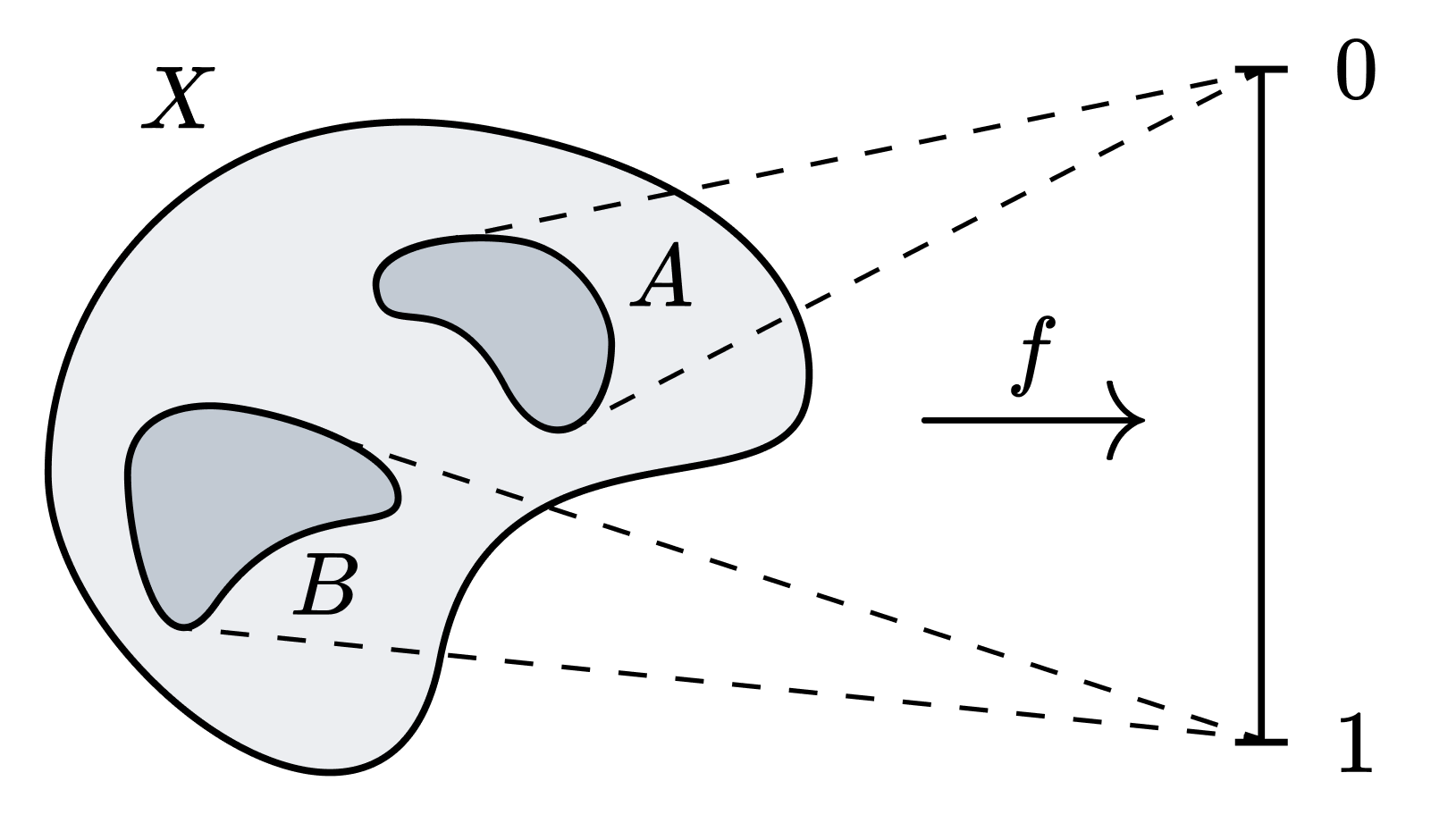
The separation axioms, e.g. normality, separate points from closed sets in the given space. The significance of the Urysohn Lemma lies in the fact that, in the case of the normal space, two closed sets can be further separated in a nice space. Specifically, with respect to an appropriate continuous map defined on the normal space to $[0, 1]$, two closed sets can be separated in $[0, 1]$. And the myriad “nice” properties of $[0, 1]$ — being a compact Hausdorff metric space, and a space which we are very familiar with and can visualise easily — suggest the remarkable potential of the Urysohn lemma.

Proof

Let us denote $Q = [0, 1] \cap \mathbb{Q}$ (actually it suffices for $Q$ to be a countable dense subset of $[0, 1]$). Since $Q$ is countable, there exists an enumeration of the elements of $Q$. For instance, consider the lexicographic enumeration of the numerators and denominators, $\prec$.

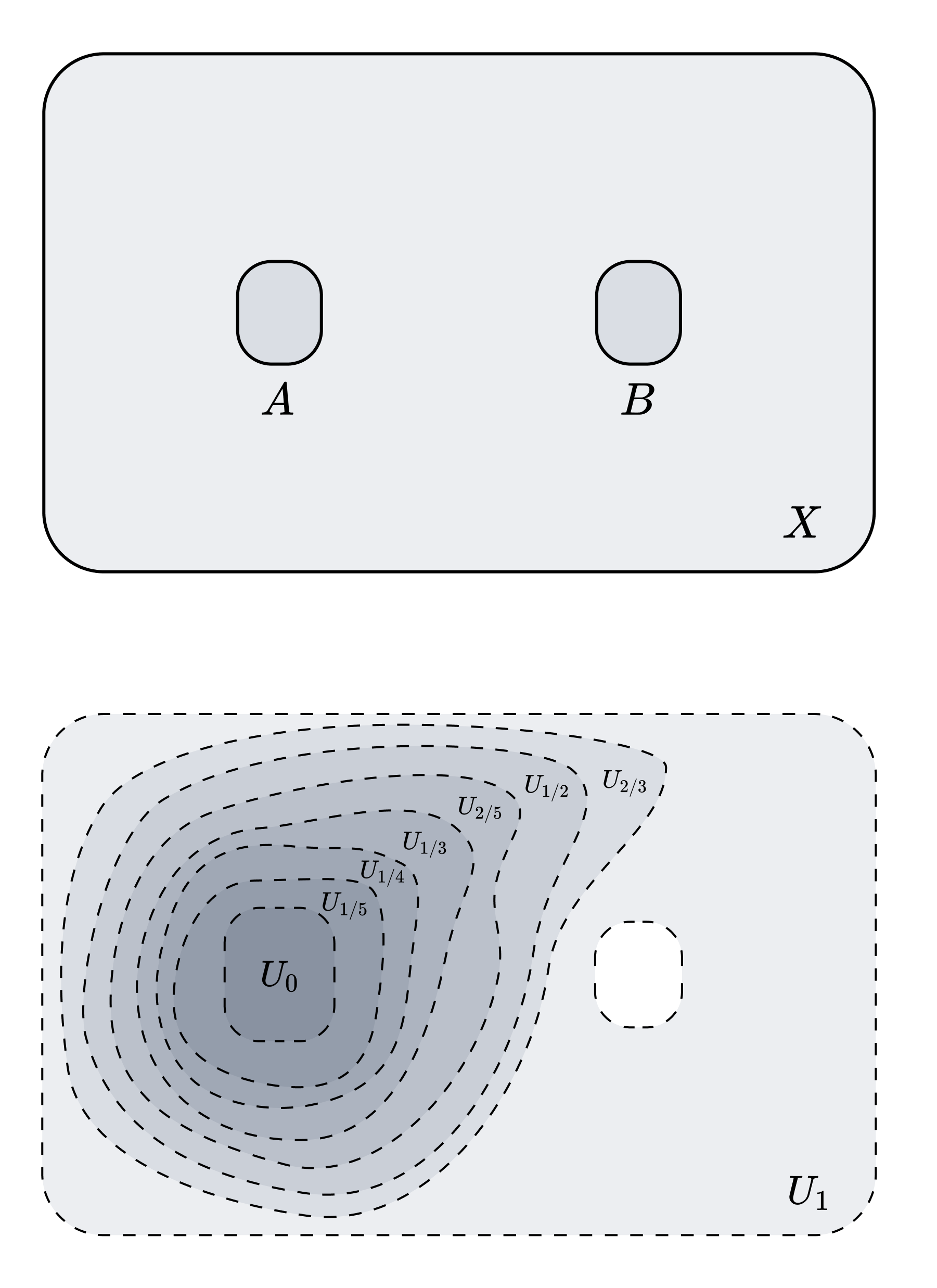
\[0 \prec 1 \prec 1/2 \prec 1/3 \prec 2/3 \prec 1/4 \prec 1/5 \prec 2/5 \prec \cdots\]

Let us now define the collection $\lbrace U_q \rbrace _{q \in Q}$. First, let $U_1 = X \setminus B$ (since $B$ is a closed set, $U_1$ is an open set). By normality, there exists an open set $U_0$ such that $A \subset U_0$ and $\overline{U_0} \subset U_1$. The remaining $U_q$ are recursively defined in the following manner. For any $p \prec q$,

• If $p < q$, then $\overline{U_p} \subset U_q$.
• If $q < p$, then $\overline{U_q} \subset U_p$.

By normality, these conditions can be satisfied, allowing us to fully define the collection $\lbrace U_q \rbrace _{q \in Q}$.

Now, let us define the function $f: X \to [0, 1]$ as follows.

\[f(x) = \begin{cases} \sup_{<}\{q \in Q : x \notin U_q \} & x \notin U_0 \\ 0 & x \in U_0 \end{cases}\]

The notation $\sup_<$ indicates that we are taking the supremum with respect to $<$ rather than $\prec$. From the definition, it follows that $f[A] = 0$ and $f[B] = 1$.

To complete the proof, we must show that $f$ is continuous. Since $\lbrace B_\epsilon(q) \cap [0, 1] : q \in Q, \epsilon \in \mathbb{Q}_{>0} \rbrace$ forms a basis for the topology on $[0, 1]$, it suffices to show that for any $q \in Q$ and postivie rational $\epsilon$ smaller than a certain supremum, the set $S_{q, \epsilon} = f^{-1}(B_\epsilon(q) \cap [0, 1])$ is an open set. Indeed,

• If $0 < q < 1$, then $S_{q, \epsilon} = (X \setminus \overline{U_{q-\epsilon}}) \cap U_{q + \epsilon}$, which is an open set.
• If $q = 0$, then $S_{0, \epsilon} = U_\epsilon$, which is an open set.
• If $q = 1$, then $S_{1, \epsilon} = X \setminus \overline{U_{1 - \epsilon}}$, which is an open set.

Thus, $f$ is continuous. ■

Remarks

• The converse of the Urysohn lemma trivially holds. That is, for any closed sets $A, B \subset X$, if there exists a continuous function $f: X \to [0, 1]$ that separates $A$ and $B$, then the sets $U = f^{-1}[0, 1/2)$ and $V = f^{-1}(1/2, 1]$ are disjoint open sets that separate $A$ and $B$, implying that $X$ is normal. In simple terms, in normal spaces, the Urysohn separation property and the separation axiom are equivalent.

• This does not hold in regular spaces. Specifically, given any closed set $F$ and point $a$ in a regular space $X$, it is not always the case that there exists a continuous function $f: X \to [0, 1]$ satisfying $f(a) = 0$ and $f[F] = \lbrace 1 \rbrace$. A regular space that is Urysohn separable is called a Tychonoff space or a completely regular space, which is a strictly stronger condition than regularity.

• The reason the proof of the Urysohn Lemma does not go through for regular spaces is that constructing the collection $\lbrace U_q \rbrace $ satisfying $p < q \implies \overline{U_p} \subset U_q$ requires the normality axiom.

Urysohn Metrisation Theorem

As an application of the Urysohn Lemma, let us prove the Urysohn Metrisation Theorem.

Urysohn Metrisation Theorem. A second countable normal space is metrizable.

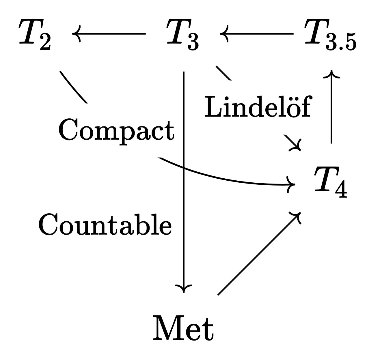
Recall that a second countable regular space is a normal space. Hence the statement of the above theorem can be strengthened to “A second countable regular space is metrisable.”

Thus, the implications between spaces can be summarised as follows. Note that the longer the arrow, the stronger the required condition. The implication $T_2 \to T_4$ is strictly more difficult than $T_3 \to T_4$, and this is evidenced by the fact that the former requires a condition — compactness — strictly stronger than the latter — Lindelöf. Similarly, $T_3 \to \mathrm{Met}$ is strictly more difficult than $T_3 \to T_4$, as the second countability required in the former is strictly stronger than the Lindelöf property. However, neither $T_2 \to T_4$ nor $T_3 \to \mathrm{Met}$ is strictly more difficult than the other (the lengths of both arrows are similar). This is again evidenced by the fact that compactness and second countability do not generally imply each other.

Proof

Let $X$ be a second countable normal space. We will prove the following lemma.

Lemma. There exists a countable collection of continuous functions $\mathcal{F}$ mapping $X$ to $[0, 1]$ such that for any point $x_0 \in X$ and its neighbourhood $U$, there exists a function $f \in \mathcal{F}$ satisfying $f(x_0) > 0$ and $f[X \setminus U] = \lbrace 0 \rbrace$.

Given $x_0$ and $U$, the existence of such an $f$ follows from the Urysohn Lemma. Our task is to reduce this to a countable collection of functions. Let $\mathcal{B} = \lbrace B_n \rbrace $ be a countable basis for the topology on $X$. When $B_m \subset B_n$, we define a continuous function $f_{nm}: X \to [0, 1]$ satisfying the following conditions according to the Urysohn Lemma:

• $f_{nm}[\overline{B_m}] = 1$
• $f_{nm}[X \setminus B_n] = 0$

Let $\mathcal{F} = \lbrace f_{nm} \rbrace $. Given any point $x_0$ and its neighbourhood $U$, by the definition of a basis, there exists a basis element $B_n$ such that $x_0 \in B_n \subset U$. Furthermore, by normality, there exists an open set $V$ such that $x \in \overline{V} \subset B_n$. Again, by the definition of a basis, there exists a basis element $B_m$ such that $x \in B_m \subset V$. Hence $f_{nm} \in \mathcal{F}$ satisfies the conditions of the lemma. □

Now, let us prove the main theorem. The idea is to embed $X$ into $[0, 1]^\omega$, as $[0, 1]^\omega$ equipped with metric topology is known to be a metric space. It then follows that $X$ is metrisable, being a space homeomorphic to a subspace of a metric space.

Let $\mathcal{F} = \lbrace f_n \mid n \in \omega \rbrace $ be the countable collection of functions given by the lemma. We define the mapping $F: X \to [0, 1]^\omega$ as follows:

\[F: x \mapsto (f_1(x), f_2(x), f_3(x), \dots)\]

We will show that $F$ is an embedding. That is, we need to demonstrate that $F$ is continuous, injective, and a homeomorphism between the domain and the image.

Since each $f_n$ is continuous, by the properties of the product topology, $F$ is continuous (side note: one can regard this as the definition of the product toplogy). The injectivity of $F$ follows from the fact that $X$ is Hausdorff. Therefore, it suffices to show the following:

If $U \subset X$ is an open set, then $F[U]$ is open in $\mathrm{im} F$.

Let us show that for any $y_0 \in F[U]$, there exists a set $V \subset F[U]$ open in $\mathrm{im} F$ that contains $y_0$. By the definition of $F[U]$, there exists some $x_0 \in X$ such that $F(x_0) = y_0$. Let $f_n \in \mathcal{F}$ be a function satisfying the conditions of the lemma for $x_0$ and $U$. Since $f_n(x_0) = 1$, it follows that $(y_0)_n = 1$. Therefore, $W = \pi_n^{-1}(0, 1] \subset [0, 1]^\omega$ is a set containing $y_0$ that is open in $[0, 1]^\omega$.

Now, we need to show that $W \cap \mathrm{im} F \subset F[U]$. For any $w \in W$, we can write $F(x_1) = w$. Additionally, if $w \in \mathrm{im} F$, then $f_n(x_1) = 1$. However, since $f_n$ vanishes outside of $U$, it follows that $x_1 \in U$. Thus, $w \in F[U]$, i.e. $W \cap \mathrm{im} F$ is contained in $F[U]$ and is an open set in $\mathrm{im} F$ containing $y_0$. Hence, $F[U]$ is an open set in $\mathrm{im} F$. ■

Remarks

• The Urysohn Metrisation Theorem can be strengthened to the Nagata-Smirnov Metrisation Theorem. The statement is as follows:

  A space $X$ is metrizable if and only if $X$ is regular and has a countably locally finite topology basis.

  A collection of subsets $\mathcal{A}$ of a topological space $X$ is said to be locally finite if for any point $x \in X$, there exists a neighbourhood $U$ such that $U$ intersects only finitely many sets from $\mathcal{A}$. A topological basis $\mathcal{B}$ is said to be countably locally finite if it can be expressed as $\mathcal{B} = \bigcup_{n \in \omega}\mathcal{B}_n$ where each $\mathcal{B}_n$ is locally finite.

• A slight modification of the proof of the Urysohn Metrisation Theorem leads to the following result.

  Theorem. Let $X$ be a $T_1$ space, and let $\lbrace f_{\alpha} \rbrace_{\alpha \in J}$ be a collection of continuous functions $f_\alpha : X \to [0, 1]$ satisfying the following condition: for any point $x_0 \in X$ and its neighbourhood $U$, there exists $\alpha \in J$ such that $f_\alpha(x_0) = 1$ and $f_\alpha[X \setminus U] = \lbrace 0 \rbrace$. Then, the mapping $F(x) = (f_\alpha(x))_{\alpha \in J}$ embeds $X$ into $[0, 1]^J$.

  Omitting the $T_1$ condition may result in $F$ not being injective. This theorem is used to prove the Stone-Čech compactification.